Keras in practice
The scene: the 40 lines from Chapter 30
In Chapter 30 we wrote a network from scratch: 40 lines of code. Forward, backward, gradient, update.
In Keras the same thing takes five lines.
This chapter teaches you how to use the library. But careful: don't skip Chapters 30 and 31. Keras is easy to use, but understanding why it isn't working is only possible if you know what's inside.
Column names
The rental data has Uzbek column names. xonalar rooms, maydon_m2 area in m², qavat floor, qavatlar_soni floors in the building, metro_km distance to the metro, mebel furnished (0/1), qurilgan_yil year built, narx_usd monthly rent in USD. The target ijaraga_berildi_30k means rented within 30 days.
The first model: five lines
import os
os.environ["CUDA_VISIBLE_DEVICES"] = "-1"       # CPU, for reproducibility
os.environ["TF_CPP_MIN_LOG_LEVEL"] = "3"
import numpy as np
import pandas as pd
import tensorflow as tf
from tensorflow import keras

tf.random.set_seed(42)
np.random.seed(42)
tf.config.threading.set_intra_op_parallelism_threads(2)
print(f"TensorFlow {tf.__version__}  |  Keras {keras.__version__}")
print(f"Device: {'GPU' if tf.config.list_physical_devices('GPU') else 'CPU'}")
TensorFlow 2.20.0  |  Keras 3.12.0
Device: CPU
from sklearn.model_selection import train_test_split
from sklearn.preprocessing import StandardScaler
from sklearn.impute import SimpleImputer

df = pd.read_csv(DATA / "uy_ijara.csv")
num = ["xonalar", "maydon_m2", "qavat", "qavatlar_soni", "metro_km", "mebel", "qurilgan_yil"]
X = SimpleImputer(strategy="median").fit_transform(df[num])
y = df["ijaraga_berildi_30k"].to_numpy(dtype="float32")

X_tr, X_te, y_tr, y_te = train_test_split(X, y, test_size=0.3, random_state=42, stratify=y)
sc = StandardScaler().fit(X_tr)
X_tr, X_te = sc.transform(X_tr).astype("float32"), sc.transform(X_te).astype("float32")

model = keras.Sequential([
    keras.layers.Input(shape=(X_tr.shape[1],)),
    keras.layers.Dense(16, activation="relu"),
    keras.layers.Dense(1, activation="sigmoid"),
])
model.compile(optimizer="adam", loss="binary_crossentropy", metrics=["accuracy"])
history = model.fit(X_tr, y_tr, epochs=40, batch_size=32, verbose=0,
                    validation_split=0.2)
loss, acc = model.evaluate(X_te, y_te, verbose=0)
print(f"Test loss: {loss:.4f}   Test accuracy: {acc:.4f}")
Test loss: 0.5050 Test accuracy: 0.7722
Five lines. The same job as the 40 lines in Chapter 30.
The structure of a Sequential
model.summary(print_fn=lambda s: print(" " + s))
  Model: "sequential"
┏━━━━━━━━━━━━━━━━━━━━━━━━━━━━━━━━━┳━━━━━━━━━━━━━━━━━━━━━━━━┳━━━━━━━━━━━━━━━┓
┃ Layer (type)                    ┃ Output Shape           ┃       Param # ┃
┡━━━━━━━━━━━━━━━━━━━━━━━━━━━━━━━━━╇━━━━━━━━━━━━━━━━━━━━━━━━╇━━━━━━━━━━━━━━━┩
│ dense (Dense)                   │ (None, 16)             │           128 │
├─────────────────────────────────┼────────────────────────┼───────────────┤
│ dense_1 (Dense)                 │ (None, 1)              │            17 │
└─────────────────────────────────┴────────────────────────┴───────────────┘
 Total params: 437 (1.71 KB)
 Trainable params: 145 (580.00 B)
 Non-trainable params: 0 (0.00 B)
 Optimizer params: 292 (1.14 KB)
Let's check the Param # column against the matrix shapes from Chapter 12:
n_in = X_tr.shape[1]
print(f"Layer 1: Dense(16)")
print(f"  W shape: ({n_in}, 16) -> {n_in * 16} parameters")
print(f"  b shape: (16,)            -> 16 parameters")
print(f"  total: {n_in * 16 + 16}")
print()
print(f"Layer 2: Dense(1)")
print(f"  W: (16, 1) -> 16  |  b: (1,) -> 1  |  total: 17")
print()
print(f"Overall: {n_in * 16 + 16 + 17}")
print(f"model.count_params(): {model.count_params()}")
Layer 1: Dense(16)
  W shape: (7, 16) -> 112 parameters
  b shape: (16,)            -> 16 parameters
  total: 128

Layer 2: Dense(1)
  W: (16, 1) -> 16  |  b: (1,) -> 1  |  total: 17

Overall: 145
model.count_params(): 145
Three steps: build, compile, fit
show(pd.DataFrame([
    {"Step": "1. Build", "What you do": "The layers and their shapes",
     "In code": "keras.Sequential([...])"},
    {"Step": "2. Compile", "What you do": "The optimizer, the loss, the metrics",
     "In code": "model.compile(...)"},
    {"Step": "3. Fit", "What you do": "The data, the epochs, the batch",
     "In code": "model.fit(...)"},
]))
| Step | What you do | In code |
|---|---|---|
| 1. Build | The layers and their shapes | keras.Sequential([...]) |
| 2. Compile | The optimizer, the loss, the metrics | model.compile(...) |
| 3. Fit | The data, the epochs, the batch | model.fit(...) |
The place where people go wrong most is the pairing of the output layer and the loss function:
show(pd.DataFrame([
    {"Task": "Binary classification", "Output layer": "Dense(1, activation='sigmoid')",
     "loss": "binary_crossentropy", "metrics": "accuracy, AUC"},
    {"Task": "Multiclass (3+ classes)", "Output layer": "Dense(n_classes, activation='softmax')",
     "loss": "sparse_categorical_crossentropy", "metrics": "accuracy"},
    {"Task": "Multilabel (several labels)", "Output layer": "Dense(n, activation='sigmoid')",
     "loss": "binary_crossentropy", "metrics": "accuracy"},
    {"Task": "Regression", "Output layer": "Dense(1): NO activation",
     "loss": "mse or mae", "metrics": "mae, RootMeanSquaredError"},
]))
| Task | Output layer | loss | metrics |
|---|---|---|---|
| Binary classification | Dense(1, activation='sigmoid') | binary_crossentropy | accuracy, AUC |
| Multiclass (3+ classes) | Dense(n_classes, activation='softmax') | sparse_categorical_crossentropy | accuracy |
| Multilabel (several labels) | Dense(n, activation='sigmoid') | binary_crossentropy | accuracy |
| Regression | Dense(1): NO activation | mse or mae | mae, RootMeanSquaredError |
softmax + binary_crossentropy: a silent mistake
This pairing doesn't raise an error; the code runs, but the model doesn't learn, or learns very badly.
The rule: sigmoid -> binary_crossentropy. softmax -> categorical_crossentropy. Regression -> no activation + mse.
One more: sparse_categorical_crossentropy is for labels that are integers (0, 1, 2), categorical_crossentropy for one-hot labels. Mix them up and you get a shape error.
print("A regression problem, three variants:")
yn = df["narx_usd"].to_numpy(dtype="float32")
Xn_tr, Xn_te, yn_tr, yn_te = train_test_split(X, yn, test_size=0.3, random_state=42)
scn = StandardScaler().fit(Xn_tr)
Xn_tr, Xn_te = scn.transform(Xn_tr).astype("float32"), scn.transform(Xn_te).astype("float32")

print(f"  (the average rent is {yn.mean():.0f} USD: the MAE MUST be far below that)")
print()
print(f"{'variant':<34} {'epochs':>6} {'test MAE':>10}")
print("-" * 54)
for name, last, ep in [
    ("Dense(1): right, few epochs", keras.layers.Dense(1), 30),
    ("Dense(1): right, enough epochs", keras.layers.Dense(1), 400),
    ("Dense(1, 'sigmoid'): WRONG", keras.layers.Dense(1, activation="sigmoid"), 400),
]:
    tf.random.set_seed(42)
    m = keras.Sequential([keras.layers.Input(shape=(Xn_tr.shape[1],)),
                          keras.layers.Dense(32, activation="relu"), last])
    m.compile(optimizer="adam", loss="mse", metrics=["mae"])
    m.fit(Xn_tr, yn_tr, epochs=ep, batch_size=32, verbose=0)
    _, mae = m.evaluate(Xn_te, yn_te, verbose=0)
    print(f"{name:<34} {ep:>6} {mae:>10.1f}")
A regression problem, three variants:
  (the average rent is 776 USD: the MAE MUST be far below that)

variant                            epochs   test MAE
------------------------------------------------------
Dense(1): right, few epochs            30      726.3
Dense(1): right, enough epochs        400       70.2
Dense(1, 'sigmoid'): WRONG            400      785.7
The table gives two lessons, and I missed the first one at first.
Lesson 1: too few epochs also looks like a mistake. The right architecture at 30 epochs gives an MAE close to the average rent, which means the model hasn't learned anything yet. At 400 epochs the MAE drops more than tenfold and approaches the Ridge result from Chapter 15.
In other words, while trying to show "sigmoid is bad", I had actually undertrained both models, and the gap looked small.
Lesson 2: sigmoid never recovers. Even at 400 epochs its MAE stays at the level of the average rent. The reason is clear: sigmoid squeezes the output between 0 and 1, while rents run from 225 to 1515. However long the model trains, it can't reach that range.
A bad result has two different causes, and you have to tell them apart
The three rows above show it:
| Cause | Sign | Fix |
|---|---|---|
| Undertrained | the train loss is still falling | More epochs, a larger lr |
| Wrong architecture | the train loss has stopped, but it's high | Fix the output layer/loss |
How to tell: look at the train loss curve. If it's still going down, it needs time. If it has flattened and the result is still bad, the structure is wrong.
I drew a conclusion without checking that difference. The rule from Chapter 11 applies here too: first the diagnosis, then the action.
Keras numbers come out SLIGHTLY different every time
Run the table above twice and the MAE values won't be identical: they usually differ by 1-2%.
I checked this by measuring: even with tf.random.set_seed(42), np.random.seed(42) and tf.config.experimental.enable_op_determinism(), TensorFlow didn't give the same result.
PyTorch (Chapter 31), on the other hand, reproduces exactly with torch.manual_seed(42): the same to six decimal places.
This has a practical consequence, and it applies to this book too: I didn't copy the exact numbers from this chapter into the text. Look at the table: it's recomputed on every build. The text only states the direction ("drops tenfold"), not an exact number.
Do the same: when you report a Keras result, don't give one number; give the mean and spread of several runs (the rule from Chapter 10).
Callbacks: steering the training
tf.random.set_seed(42)
model2 = keras.Sequential([
    keras.layers.Input(shape=(X_tr.shape[1],)),
    keras.layers.Dense(64, activation="relu"),
    keras.layers.Dropout(0.3),
    keras.layers.Dense(32, activation="relu"),
    keras.layers.Dense(1, activation="sigmoid"),
])
model2.compile(optimizer=keras.optimizers.Adam(1e-3),
               loss="binary_crossentropy", metrics=["accuracy"])

callbacks = [
    keras.callbacks.EarlyStopping(monitor="val_loss", patience=15, restore_best_weights=True),
    keras.callbacks.ReduceLROnPlateau(monitor="val_loss", factor=0.3, patience=7, min_lr=1e-5),
]
t2 = model2.fit(X_tr, y_tr, epochs=300, batch_size=32, verbose=0,
                validation_split=0.2, callbacks=callbacks)
print(f"Epochs allowed           : 300")
print(f"Early stopping stopped at: {len(t2.history['loss'])} epochs")
print(f"Best val_loss            : {min(t2.history['val_loss']):.4f}")
loss2, acc2 = model2.evaluate(X_te, y_te, verbose=0)
print(f"Test accuracy            : {acc2:.4f}")
Epochs allowed           : 300
Early stopping stopped at: 18 epochs
Best val_loss            : 0.6136
Test accuracy            : 0.7722
show(pd.DataFrame([
    {"Callback": "EarlyStopping", "What it does": "Stops when val_loss stops improving",
     "Key parameter": "patience, restore_best_weights=True"},
    {"Callback": "ReduceLROnPlateau", "What it does": "Lowers the learning rate on a plateau",
     "Key parameter": "factor, patience"},
    {"Callback": "ModelCheckpoint", "What it does": "Saves the best model to disk",
     "Key parameter": "save_best_only=True"},
    {"Callback": "TensorBoard", "What it does": "Writes charts to a log",
     "Key parameter": "log_dir"},
]))
| Callback | What it does | Key parameter |
|---|---|---|
| EarlyStopping | Stops when val_loss stops improving | patience, restore_best_weights=True |
| ReduceLROnPlateau | Lowers the learning rate on a plateau | factor, patience |
| ModelCheckpoint | Saves the best model to disk | save_best_only=True |
| TensorBoard | Writes charts to a log | log_dir |
Don't forget restore_best_weights=True
By default EarlyStopping keeps the last weights: the model that got worse over the patience epochs.
restore_best_weights=True goes back to the best epoch. You almost always want this, but it's off by default.
Training curves: the most important diagnostic
import matplotlib.pyplot as plt

figure, axes = plt.subplots(1, 2, figsize=(13.5, 4.6))
axes[0].plot(t2.history["loss"], lw=2, label="train", color="#1a73e8")
axes[0].plot(t2.history["val_loss"], lw=2, label="validation", color="#c5221f")
axes[0].set_xlabel("Epoch"); axes[0].set_ylabel("Loss")
axes[0].set_title("Loss", fontweight="bold"); axes[0].legend(); axes[0].grid(alpha=.3)

axes[1].plot(t2.history["accuracy"], lw=2, label="train", color="#1a73e8")
axes[1].plot(t2.history["val_accuracy"], lw=2, label="validation", color="#c5221f")
axes[1].set_xlabel("Epoch"); axes[1].set_ylabel("Accuracy")
axes[1].set_title("Accuracy", fontweight="bold"); axes[1].legend(); axes[1].grid(alpha=.3)
fig("keras_tarix.png", caption="If the two lines pull apart, it's overfitting. If they run side by side, it's good.")

last_gap = t2.history["val_loss"][-1] - t2.history["loss"][-1]
print(f"At the last epoch val_loss - loss = {last_gap:+.4f}")
print("Diagnosis:", "a sign of overfitting" if last_gap > 0.1 else "the lines are close: good")
At the last epoch val_loss - loss = +0.0725
Diagnosis: the lines are close: good
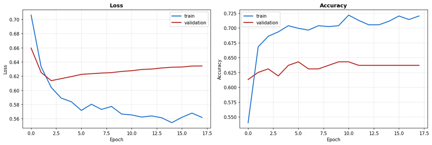
If the two lines pull apart, it's overfitting. If they run side by side, it's good.
This chart is the same idea as the learning curve in Chapter 11: look at train and validation side by side.
The Functional API: when the network isn't a straight line
Sequential only knows a linear sequence. If you need two inputs or two outputs, use the Functional API.
tf.random.set_seed(42)
inp = keras.layers.Input(shape=(X_tr.shape[1],), name="features")
h = keras.layers.Dense(32, activation="relu")(inp)
h = keras.layers.Dense(16, activation="relu")(h)
out_class = keras.layers.Dense(1, activation="sigmoid", name="goes_fast")(h)
out_price = keras.layers.Dense(1, name="price")(h)

two_outputs = keras.Model(inp, [out_class, out_price])
two_outputs.compile(
    optimizer="adam",
    loss={"goes_fast": "binary_crossentropy", "price": "mse"},
    loss_weights={"goes_fast": 1.0, "price": 0.0001},
    metrics={"goes_fast": "accuracy", "price": "mae"},
)
yn_tr2 = df["narx_usd"].to_numpy(dtype="float32")[
    train_test_split(np.arange(len(df)), test_size=0.3, random_state=42, stratify=y)[0]]
t3 = two_outputs.fit(X_tr, {"goes_fast": y_tr, "price": yn_tr2},
                     epochs=40, batch_size=32, verbose=0, validation_split=0.2)
result = two_outputs.evaluate(X_te, {"goes_fast": y_te,
                                     "price": df["narx_usd"].to_numpy(dtype="float32")[
                                         train_test_split(np.arange(len(df)), test_size=0.3,
                                                          random_state=42, stratify=y)[1]]},
                              verbose=0, return_dict=True)
print("One network, TWO tasks:")
for k, v in result.items():
    print(f"  {k:28s} {v:.4f}")
One network, TWO tasks:
  goes_fast_accuracy           0.7500
  goes_fast_loss               0.5325
  loss                         3.6039
  price_loss                   30369.9316
  price_mae                    146.5417
One network learned two things at once: whether a flat goes fast and what it costs. The hidden layers serve both.
When you need the Functional API
- Several inputs (for example image + text)
- Several outputs (the example above)
- Splitting or merging layers (the skip connection in ResNet)
- Transfer learning: connecting into the middle of an existing model
Sequential stays for the simple cases.
tf.data: feeding data efficiently
import time
batch = 64
ds_tr = (tf.data.Dataset.from_tensor_slices((X_tr, y_tr))
         .shuffle(1000, seed=42).batch(batch).prefetch(tf.data.AUTOTUNE))
ds_te = tf.data.Dataset.from_tensor_slices((X_te, y_te)).batch(batch)

tf.random.set_seed(42)
m4 = keras.Sequential([keras.layers.Input(shape=(X_tr.shape[1],)),
                       keras.layers.Dense(32, activation="relu"),
                       keras.layers.Dense(1, activation="sigmoid")])
m4.compile(optimizer="adam", loss="binary_crossentropy", metrics=["accuracy"])
t0 = time.perf_counter(); m4.fit(ds_tr, epochs=30, verbose=0); dt_ds = time.perf_counter()-t0
print(f"With tf.data      : {dt_ds:.1f}s, test accuracy {m4.evaluate(ds_te, verbose=0)[1]:.4f}")

tf.random.set_seed(42)
m5 = keras.Sequential([keras.layers.Input(shape=(X_tr.shape[1],)),
                       keras.layers.Dense(32, activation="relu"),
                       keras.layers.Dense(1, activation="sigmoid")])
m5.compile(optimizer="adam", loss="binary_crossentropy", metrics=["accuracy"])
t0 = time.perf_counter(); m5.fit(X_tr, y_tr, batch_size=batch, epochs=30, verbose=0); dt_np = time.perf_counter()-t0
print(f"With a numpy array: {dt_np:.1f}s, test accuracy {m5.evaluate(X_te, y_te, verbose=0)[1]:.4f}")
print()
print("On small data there's no difference. You need tf.data on big data:")
print("  - when it doesn't all fit in memory (streaming from disk)")
print("  - when you need image augmentation")
print("  - so the GPU isn't left waiting, thanks to prefetch")
With tf.data      : 0.5s, test accuracy 0.7750
With a numpy array: 1.0s, test accuracy 0.7806

On small data there's no difference. You need tf.data on big data:
  - when it doesn't all fit in memory (streaming from disk)
  - when you need image augmentation
  - so the GPU isn't left waiting, thanks to prefetch
Saving and loading a model
path = ISH / "model.keras"
model2.save(path)
print(f"Saved: {path.name}  ({path.stat().st_size / 1024:.0f} KB)")

loaded = keras.models.load_model(path)
a1 = model2.predict(X_te[:5], verbose=0).ravel()
a2 = loaded.predict(X_te[:5], verbose=0).ravel()
print(f"Original model's predictions: {a1.round(5)}")
print(f"The loaded model            : {a2.round(5)}")
print(f"Exactly the same            : {bool(np.allclose(a1, a2))}")
Saved: model.keras  (58 KB)
Original model's predictions: [0.32769 0.64991 0.66323 0.19593 0.7781 ]
The loaded model            : [0.32769 0.64991 0.66323 0.19593 0.7781 ]
Exactly the same            : True
Saving the model doesn't save the StandardScaler
model.save() saves only the network. The scaler, imputer and encoder: none of them are inside it.
If the model on the server gets data at the wrong scale, its predictions become meaningless, and it raises no error.
The fix: save the preprocessing steps separately (joblib.dump(scaler, ...)), or put the normalisation inside the network with keras.layers.Normalization.
We come back to this in Chapter 40.
import joblib
sc_path = ISH / "scaler.joblib"
joblib.dump(sc, sc_path)
print(f"Scaler saved separately: {sc_path.name} ({sc_path.stat().st_size} bytes)")
print()
# or we put the normalisation INSIDE the network
tf.random.set_seed(42)
norm = keras.layers.Normalization()
X_raw_tr = SimpleImputer(strategy="median").fit_transform(df[num])[
    train_test_split(np.arange(len(df)), test_size=0.3, random_state=42, stratify=y)[0]]
norm.adapt(X_raw_tr.astype("float32"))
inner = keras.Sequential([keras.layers.Input(shape=(len(num),)), norm,
                          keras.layers.Dense(32, activation="relu"),
                          keras.layers.Dense(1, activation="sigmoid")])
inner.compile(optimizer="adam", loss="binary_crossentropy", metrics=["accuracy"])
inner.fit(X_raw_tr.astype("float32"), y_tr, epochs=40, batch_size=32, verbose=0)
X_raw_te = SimpleImputer(strategy="median").fit_transform(df[num])[
    train_test_split(np.arange(len(df)), test_size=0.3, random_state=42, stratify=y)[1]]
print("Normalisation INSIDE the network: it's given RAW data:")
print(f"  test accuracy: {inner.evaluate(X_raw_te.astype('float32'), y_te, verbose=0)[1]:.4f}")
print("  Save this model and the scaling is saved along with it.")
Scaler saved separately: scaler.joblib (767 bytes)

Normalisation INSIDE the network: it's given RAW data:
  test accuracy: 0.7750
  Save this model and the scaling is saved along with it.
Keras vs sklearn: a comparison
from sklearn.ensemble import RandomForestClassifier
from sklearn.linear_model import LogisticRegression
from sklearn.model_selection import cross_val_score

print(f"{'model':<34} {'test accuracy':>14}")
print("-" * 50)
print(f"{'Keras MLP (64-32, dropout)':<34} {acc2:>14.4f}")
for name, m in [("LogisticRegression", LogisticRegression(max_iter=3000)),
                ("RandomForest", RandomForestClassifier(n_estimators=200, random_state=42))]:
    m.fit(X_tr, y_tr)
    print(f"{name:<34} {m.score(X_te, y_te):>14.4f}")
model                               test accuracy
--------------------------------------------------
Keras MLP (64-32, dropout)                 0.7722
LogisticRegression                         0.7694
RandomForest                               0.7250
The conclusion from Chapter 30 still holds: on tabular data Keras gives no advantage.
What we learned today
show(pd.DataFrame([
    {"Concept": "Three steps", "In one sentence": "Sequential -> compile -> fit"},
    {"Concept": "Output and loss pairing", "In one sentence": "sigmoid+BCE, softmax+CCE, regression: no activation+MSE"},
    {"Concept": "EarlyStopping", "In one sentence": "DON'T FORGET restore_best_weights=True"},
    {"Concept": "The training curve", "In one sentence": "Train and val side by side: the main diagnostic"},
    {"Concept": "Functional API", "In one sentence": "Several inputs/outputs or a branching network"},
    {"Concept": "tf.data", "In one sentence": "For big data, augmentation, prefetch"},
    {"Concept": "The saving trap", "In one sentence": "model.save() doesn't save the scaler"},
]))
| Concept | In one sentence |
|---|---|
| Three steps | Sequential -> compile -> fit |
| Output and loss pairing | sigmoid+BCE, softmax+CCE, regression: no activation+MSE |
| EarlyStopping | DON'T FORGET restore_best_weights=True |
| The training curve | Train and val side by side: the main diagnostic |
| Functional API | Several inputs/outputs or a branching network |
| tf.data | For big data, augmentation, prefetch |
| The saving trap | model.save() doesn't save the scaler |
The next chapter does the same job in PyTorch, and we see how the two libraries differ.
Questions about this chapter?
The course, homework review and the other five books are in Uzbek. Questions in English are welcome on Telegram.