Clustering: K-Means, DBSCAN, hierarchical
The scene: "split our customers into groups"
The marketing department comes over: "We have 1200 listings. Split them into groups, and we'll write different ads for each group."
What groups? They don't know. There are no labels. You have to find them.
That's clustering. And it's fundamentally different from supervised learning: there is no right answer.
There is no "accuracy" in clustering
In Chapter 8 we had accuracy, because the truth was known. Here there is no truth.
That's why evaluating a clustering result is the hardest part. And the one most often skipped.
Column names
The data is synthetic Tashkent rental listings, and its column names are Uzbek. xonalar rooms, maydon_m2 area in m², qavat floor, qavatlar_soni floors in the building, metro_km distance to the metro, mebel furnished (0/1), qurilgan_yil year built, narx_usd monthly rent in USD, ijaraga_berildi_30k rented within 30 days.
K-Means: the most widely used method
The idea in three steps:
- Drop
Krandom centres - Assign every point to the nearest centre
- Move each centre to the mean of its group, and go back to step 2
import pandas as pd
import numpy as np
import matplotlib.pyplot as plt
from sklearn.cluster import KMeans
from sklearn.preprocessing import StandardScaler
from sklearn.impute import SimpleImputer

df = pd.read_csv(DATA / "uy_ijara.csv")
num = ["xonalar", "maydon_m2", "qavat", "qavatlar_soni", "metro_km", "mebel", "qurilgan_yil"]
X = SimpleImputer(strategy="median").fit_transform(df[num])
Xs = StandardScaler().fit_transform(X)

km = KMeans(n_clusters=4, n_init=10, random_state=42).fit(Xs)
print(f"Groups: {np.bincount(km.labels_)}")
print(f"Iterations: {km.n_iter_}")
print(f"Inertia (spread within the groups): {km.inertia_:.1f}")
Groups: [318 274 313 295]
Iterations: 36
Inertia (spread within the groups): 5304.0
You can write the algorithm by hand too; it's that simple:
def kmeans_by_hand(X, k=4, steps=20, seed=42):
    r = np.random.default_rng(seed)
    centre = X[r.choice(len(X), k, replace=False)]
    for _ in range(steps):
        dist = ((X[:, None, :] - centre[None, :, :]) ** 2).sum(axis=2)
        label = dist.argmin(axis=1)
        new = np.array([X[label == j].mean(axis=0) if (label == j).any() else centre[j]
                        for j in range(k)])
        if np.allclose(new, centre):
            break
        centre = new
    inertia = sum(((X[label == j] - centre[j]) ** 2).sum() for j in range(k))
    return label, centre, inertia

y_h, c_h, in_h = kmeans_by_hand(Xs, k=4)
print(f"Hand-written inertia  : {in_h:.1f}")
print(f"sklearn inertia       : {km.inertia_:.1f}")
print(f"Group sizes (by hand) : {np.bincount(y_h)}")
Hand-written inertia  : 5319.0
sklearn inertia       : 5304.0
Group sizes (by hand) : [294 370 257 279]
How many groups? The elbow method
You choose K. The model doesn't tell you.
inertia = []
Ks = range(1, 11)
for k in Ks:
    inertia.append(KMeans(n_clusters=k, n_init=10, random_state=42).fit(Xs).inertia_)

table = pd.DataFrame({"K": list(Ks), "inertia": [round(i, 1) for i in inertia]})
table["drop"] = [None] + [round(inertia[i-1] - inertia[i], 1) for i in range(1, len(inertia))]
show(table)
| K | inertia | drop |
|---|---|---|
| 1 | 8 400 | NaN |
| 2 | 6 754.1 | 1 645.9 |
| 3 | 5 866.8 | 887.3 |
| 4 | 5 304 | 562.8 |
| 5 | 4 918.6 | 385.4 |
| 6 | 4 599.5 | 319.1 |
| 7 | 4 344.3 | 255.2 |
| 8 | 4 109.1 | 235.3 |
| 9 | 3 914.2 | 194.9 |
| 10 | 3 739.9 | 174.3 |
from sklearn.metrics import silhouette_score

sil = []
for k in range(2, 11):
    yl = KMeans(n_clusters=k, n_init=10, random_state=42).fit_predict(Xs)
    sil.append(silhouette_score(Xs, yl))

figure, axes = plt.subplots(1, 2, figsize=(13.5, 4.5))
axes[0].plot(list(Ks), inertia, "o-", lw=2, color="#1a73e8")
axes[0].set_xlabel("K (number of groups)"); axes[0].set_ylabel("Inertia")
axes[0].set_title("The elbow method: look for the 'elbow'", fontweight="bold")
axes[0].grid(alpha=.3)

axes[1].plot(range(2, 11), sil, "o-", lw=2, color="#137333")
best_k = int(np.argmax(sil)) + 2
axes[1].axvline(best_k, ls="--", color="red", lw=1.2, label=f"highest: K={best_k}")
axes[1].set_xlabel("K"); axes[1].set_ylabel("Silhouette score")
axes[1].set_title("Silhouette: a clearer criterion", fontweight="bold")
axes[1].legend(); axes[1].grid(alpha=.3)
fig("elbow.png", caption="Left: the elbow, which may not be visible to the eye. Right: the silhouette, whose maximum is clearer.")

print(f"{'K':>4} {'silhouette':>12}")
print("-" * 18)
for k, s in zip(range(2, 11), sil):
    flag = "  <-- highest" if k == best_k else ""
    print(f"{k:>4} {s:>12.4f}{flag}")
   K   silhouette
------------------
   2       0.1797  <-- highest
   3       0.1645
   4       0.1632
   5       0.1658
   6       0.1591
   7       0.1590
   8       0.1610
   9       0.1642
  10       0.1652
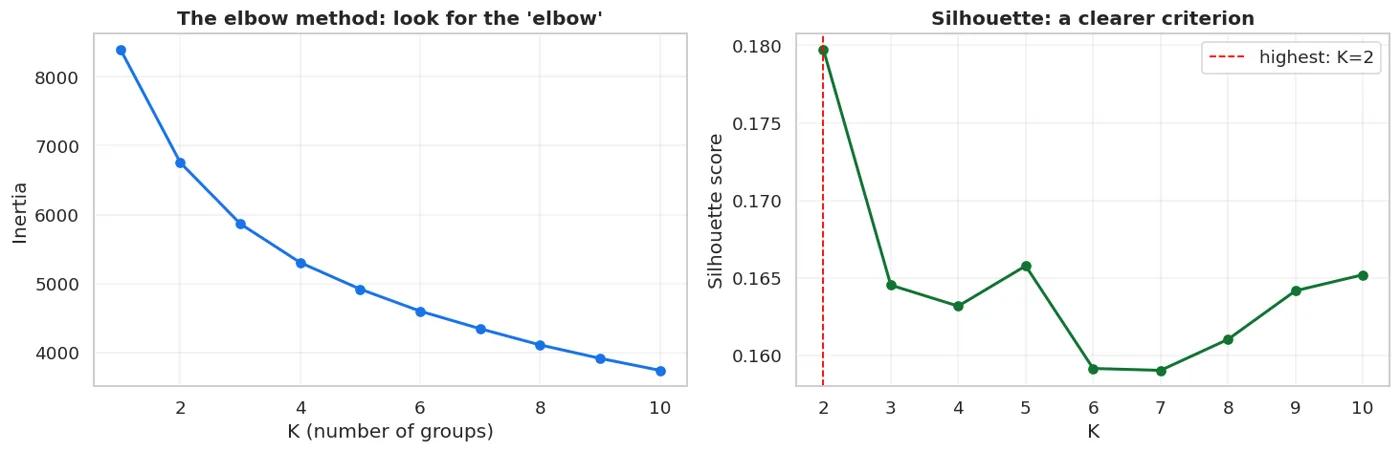
Left: the elbow, which may not be visible to the eye. Right: the silhouette, whose maximum is clearer.
The elbow often shows no elbow
Textbooks draw the elbow chart with a nice sharp bend. On real data the curve is smooth, and you can't tell where the "elbow" is.
The chart above is like that too. That's why in practice you use the silhouette: it has a clear maximum.
But the most reliable criterion is different: open the groups and read them. If the groups have no business meaning, they're useless however high the silhouette.
What the silhouette measures
print("The silhouette is computed for every point:")
print("  a = the average distance to the points in its own group")
print("  b = the average distance to the nearest OTHER group")
print("  silhouette = (b - a) / max(a, b)")
print()
show(pd.DataFrame([
    {"Value": "close to +1", "Meaning": "The point sits firmly in its group, far from the others"},
    {"Value": "around 0", "Meaning": "It's on the border between two groups"},
    {"Value": "negative", "Meaning": "It landed in the wrong group"},
]))
The silhouette is computed for every point:
  a = the average distance to the points in its own group
  b = the average distance to the nearest OTHER group
  silhouette = (b - a) / max(a, b)
| Value | Meaning |
|---|---|
| close to +1 | The point sits firmly in its group, far from the others |
| around 0 | It's on the border between two groups |
| negative | It landed in the wrong group |
from sklearn.metrics import silhouette_samples
km_best = KMeans(n_clusters=best_k, n_init=10, random_state=42).fit(Xs)  # best_k is the K with the highest silhouette
samples = silhouette_samples(Xs, km_best.labels_)
ana = pd.DataFrame({"group": km_best.labels_, "silhouette": samples})
g = ana.groupby("group").silhouette.agg(["size", "mean", "min"]).round(4)
g.columns = ["rows", "mean sil", "lowest sil"]
show(g.reset_index())
print()
print(f"Rows with a negative silhouette: {int((samples < 0).sum())} / {len(samples)}")
Rows with a negative silhouette: 5 / 1200
| group | rows | mean sil | lowest sil |
|---|---|---|---|
| 0 | 564 | 0.16 | -0.013 |
| 1 | 636 | 0.198 | 0.015 |
READING the groups: the most important step
Numbers aren't enough. What do the groups mean?
result = df[num].copy()
result["group"] = km_best.labels_
summary = result.groupby("group").agg({
    "xonalar": "mean", "maydon_m2": "mean", "metro_km": "mean",
    "mebel": "mean", "qurilgan_yil": "mean",
}).round(2)
summary["rows"] = result.groupby("group").size()
show(summary.reset_index())
print()
print("Also: do the groups differ in price and in renting fast?")
check = df.assign(group=km_best.labels_).groupby("group").agg({
    "narx_usd": "mean", "ijaraga_berildi_30k": "mean"}).round(3)
show(check.reset_index())
Also: do the groups differ in price and in renting fast?
| group | xonalar | maydon_m2 | metro_km | mebel | qurilgan_yil | rows |
|---|---|---|---|---|---|---|
| 0 | 3.48 | 74.36 | 2.69 | 0.6 | 1 999.24 | 564 |
| 1 | 1.65 | 41.96 | 2.5 | 0.62 | 1 998.7 | 636 |
| group | narx_usd | ijaraga_berildi_30k |
|---|---|---|
| 0 | 955.922 | 0.271 |
| 1 | 616.635 | 0.715 |
The group means differ from each other, so you could give them names: "small cheap flats", "central and furnished" and so on.
But here I have to stop and give an honest assessment.
Let's look at the silhouette scores: the highest is 0.1797 (at K=2), and at K=4 it's 0.1632. Those are low scores.
show(pd.DataFrame([
    {"Silhouette": "above 0.70", "Meaning": "Strong, clearly separated groups"},
    {"Silhouette": "0.50 - 0.70", "Meaning": "A reliable structure"},
    {"Silhouette": "0.25 - 0.50", "Meaning": "A weak structure: be careful"},
    {"Silhouette": "below 0.25", "Meaning": "Considered to have NO natural groups"},
]))
| Silhouette | Meaning |
|---|---|
| above 0.70 | Strong, clearly separated groups |
| 0.50 - 0.70 | A reliable structure |
| 0.25 - 0.50 | A weak structure: be careful |
| below 0.25 | Considered to have NO natural groups |
Our score of 0.18 falls in the last row.
The conclusion: this data has no clear natural groups. K-Means drew 4 groups anyway, because that's what we asked for, and it will split any data into K pieces. The scores say that split is artificial.
The honest answer for the marketing department is:
"No natural segments were found in the data. If you need segmentation, set it with a business rule (for example, splitting by price into three), which will be more reliable than clustering."
K-Means ALWAYS returns a result, even when there are no groups
This is the most dangerous property in clustering. KMeans(n_clusters=4) never says "no groups found". It splits any data into four, even a uniform random cloud.
So always compute the silhouette and put it in the report. Without it you might present a random split as "customer segments".
As proof: K-Means "finds" groups even in random noise; below we measure that and compare it with our own result.
r_n = np.random.default_rng(1)
noise_data = r_n.normal(size=(1200, 7))      # COMPLETELY random
km_n = KMeans(n_clusters=4, n_init=10, random_state=42).fit(noise_data)
print("K-Means on COMPLETELY RANDOM data:")
print(f"  group sizes : {np.bincount(km_n.labels_)}")
print(f"  silhouette  : {silhouette_score(noise_data, km_n.labels_):.4f}")
print()
print(f"On our real data (K={best_k}): {silhouette_score(Xs, km_best.labels_):.4f}")
print()
ratio = silhouette_score(Xs, km_best.labels_) / silhouette_score(noise_data, km_n.labels_)
print(f"Ratio: our score is {ratio:.1f} times higher than chance")
K-Means on COMPLETELY RANDOM data:
  group sizes : [277 306 305 312]
  silhouette  : 0.0961

On our real data (K=2): 0.1797

Ratio: our score is 1.9 times higher than chance
The work isn't done until the group has a name
If you can't name a group in two words, it isn't a group: it's a random collection.
So the sequence is: choose K -> read the groups -> name them -> if you can't name them, change K.
The limitations of K-Means
from sklearn.datasets import make_moons, make_blobs

r = np.random.default_rng(42)
# 1) half-moon shapes
X_moon, y_moon = make_moons(n_samples=400, noise=.06, random_state=42)
# 2) groups of different sizes
X_s, y_s = make_blobs(n_samples=[400, 60, 60], centers=[[0,0],[4,4],[-4,4]],
                      cluster_std=[1.4, .4, .4], random_state=42)

figure, axes = plt.subplots(2, 2, figsize=(12, 8))
for j, (Xd, name) in enumerate([(X_moon, "Half moons"), (X_s, "Different sizes")]):
    Xd_s = StandardScaler().fit_transform(Xd)
    km_t = KMeans(n_clusters=2 if j == 0 else 3, n_init=10, random_state=42).fit_predict(Xd_s)
    axes[j, 0].scatter(Xd[:, 0], Xd[:, 1], c=km_t, cmap="viridis", s=18, alpha=.8)
    axes[j, 0].set_title(f"{name}: K-Means", fontweight="bold")
    from sklearn.cluster import DBSCAN
    db_t = DBSCAN(eps=.3 if j == 0 else .5, min_samples=5).fit_predict(Xd_s)
    axes[j, 1].scatter(Xd[:, 0], Xd[:, 1], c=db_t, cmap="viridis", s=18, alpha=.8)
    axes[j, 1].set_title(f"{name}: DBSCAN", fontweight="bold")
    for a in axes[j]: a.grid(alpha=.3)
fig("kmeans_cheklov.png", caption="K-Means expects round groups of equal size. DBSCAN finds any shape.")
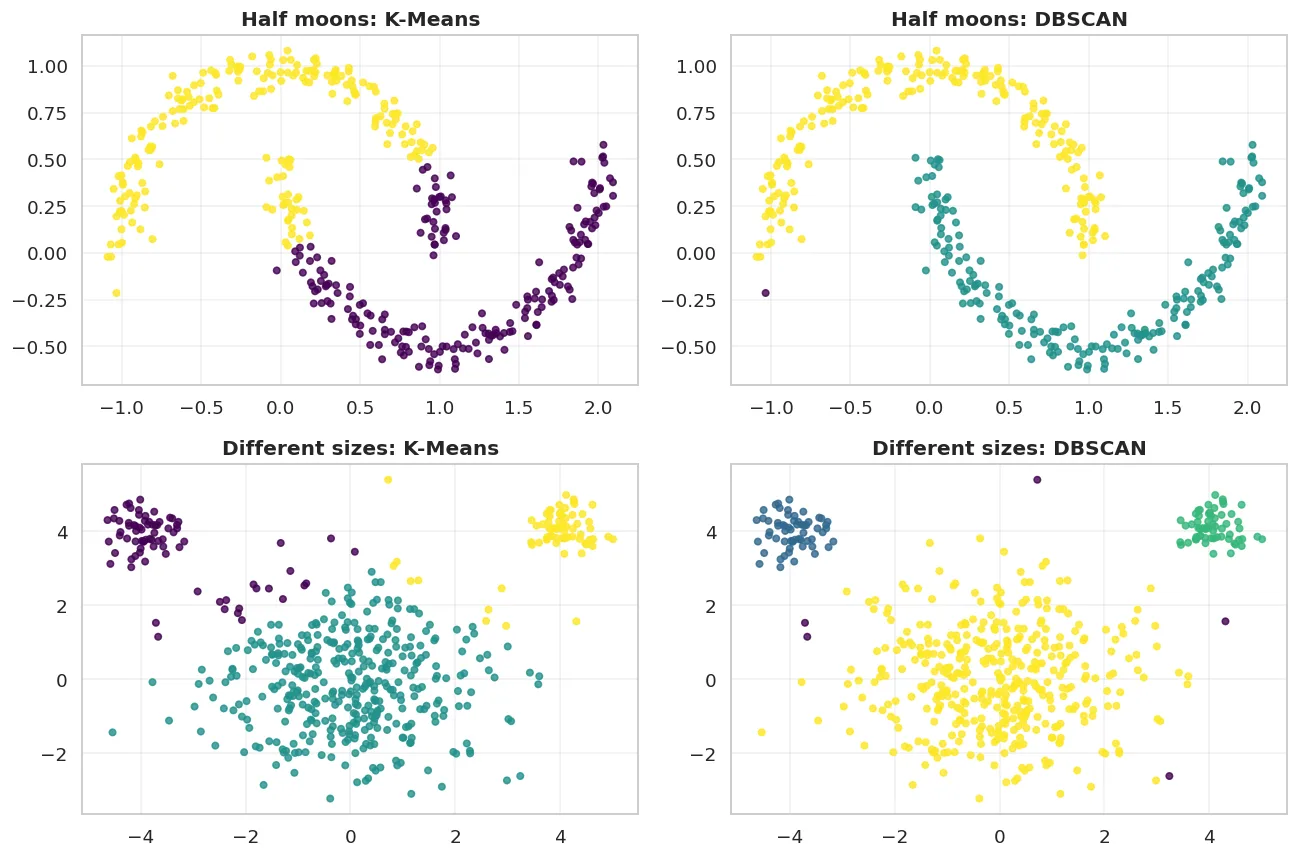
K-Means expects round groups of equal size. DBSCAN finds any shape.
show(pd.DataFrame([
    {"Limitation": "Expects round shapes", "Consequence": "Can't split half moons or rings"},
    {"Limitation": "You provide K", "Consequence": "The wrong K -> meaningless groups"},
    {"Limitation": "Expects equal sizes", "Consequence": "Folds a small group into a big one"},
    {"Limitation": "Sensitive to outliers", "Consequence": "One distant point drags a centre"},
    {"Limitation": "Depends on the starting centres", "Consequence": "That's why n_init=10 is needed"},
]))
| Limitation | Consequence |
|---|---|
| Expects round shapes | Can't split half moons or rings |
| You provide K | The wrong K -> meaningless groups |
| Expects equal sizes | Folds a small group into a big one |
| Sensitive to outliers | One distant point drags a centre |
| Depends on the starting centres | That's why n_init=10 is needed |
print("The effect of the starting centres, and the role of n_init:")
print(f"{'n_init':>8} {'inertia':>12} {'distinct results':>22}")
print("-" * 46)
for ni in [1, 3, 10]:
    results = set()
    inertias = []
    for seed in range(8):
        k_t = KMeans(n_clusters=4, n_init=ni, random_state=seed).fit(Xs)
        inertias.append(round(k_t.inertia_, 1))
        results.add(round(k_t.inertia_, 1))
    print(f"{ni:>8} {np.mean(inertias):>12.1f} {len(results):>22}")
The effect of the starting centres, and the role of n_init:
  n_init      inertia       distinct results
----------------------------------------------
       1       5377.9                      8
       3       5304.7                      6
      10       5304.1                      3
With n_init=1, different seeds give different results. n_init=10 tries 10 times and picks the best, which is why it's on by default.
DBSCAN: based on density
DBSCAN asks a different question: "does this point have enough neighbours around it?"
from sklearn.cluster import DBSCAN

print(f"{'eps':>6} {'min_samples':>12} {'groups':>10} {'noise':>9} {'silhouette':>12}")
print("-" * 54)
for eps in [0.5, 0.8, 1.2, 1.8]:
    db = DBSCAN(eps=eps, min_samples=10).fit(Xs)
    n_groups = len(set(db.labels_)) - (1 if -1 in db.labels_ else 0)
    noise = int((db.labels_ == -1).sum())
    if n_groups > 1:
        mask = db.labels_ != -1
        s = silhouette_score(Xs[mask], db.labels_[mask]) if mask.sum() > n_groups else float("nan")
    else:
        s = float("nan")
    print(f"{eps:>6} {10:>12} {n_groups:>10} {noise:>9} {s:>12.4f}")
   eps  min_samples     groups     noise   silhouette
------------------------------------------------------
   0.5           10          0      1200          nan
   0.8           10          2      1180       0.6764
   1.2           10          3       324       0.1449
   1.8           10          2         7       0.1634
DBSCAN has two advantages:
- You don't give
K: it finds the number of groups itself - It separates noise: points that belong to no group get the label
-1
But it has a cost too: choosing eps is no easier than choosing K.
DBSCAN doesn't work in high dimensions
DBSCAN relies on distance, so the curse of dimensionality from Chapter 21 hits it fully.
Once there are more than 10-15 columns, finding eps becomes almost impossible: every point looks equally far away.
So in practice the order is: first bring it down to 2-10 dimensions with PCA (Chapter 27), then DBSCAN.
Hierarchical: as a tree
from sklearn.cluster import AgglomerativeClustering
from scipy.cluster.hierarchy import dendrogram, linkage

sample = Xs[np.random.default_rng(42).choice(len(Xs), 60, replace=False)]
Z = linkage(sample, method="ward")

figure, ax = plt.subplots(figsize=(11, 4.5))
dendrogram(Z, ax=ax, no_labels=True, color_threshold=7)
ax.set_xlabel("Samples"); ax.set_ylabel("Merge distance")
ax.set_title("A dendrogram: how the groups merge", fontweight="bold")
fig("dendrogram.png", caption="From the bottom up: every point starts in its own group, then they merge step by step. A horizontal cut gives you K.")

print(f"{'K':>4} {'silhouette (ward)':>20}")
print("-" * 26)
for k in [2, 3, 4, 5, 6]:
    yl = AgglomerativeClustering(n_clusters=k, linkage="ward").fit_predict(Xs)
    print(f"{k:>4} {silhouette_score(Xs, yl):>20.4f}")
   K    silhouette (ward)
--------------------------
   2               0.1356
   3               0.1465
   4               0.1144
   5               0.1143
   6               0.1114
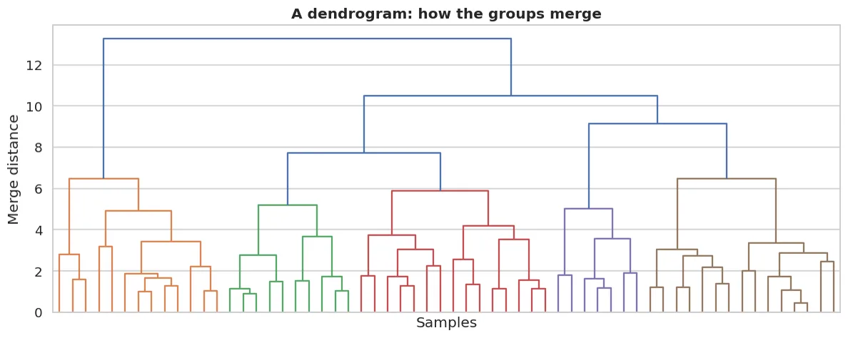
From the bottom up: every point starts in its own group, then they merge step by step. A horizontal cut gives you K.
The dendrogram's advantage: you don't give K in advance: you look at the tree, then choose where to cut.
Comparing the three
import time
from sklearn.metrics import calinski_harabasz_score, davies_bouldin_score

print(f"{'method':<28} {'groups':>9} {'silhouette':>12} {'Calinski-H':>12} {'time':>8}")
print("-" * 76)
for name, model in [
    ("KMeans(4)", KMeans(n_clusters=4, n_init=10, random_state=42)),
    ("DBSCAN(eps=1.2)", DBSCAN(eps=1.2, min_samples=10)),
    ("Agglomerative(4)", AgglomerativeClustering(n_clusters=4, linkage="ward")),
]:
    t0 = time.perf_counter()
    yl = model.fit_predict(Xs)
    dt = time.perf_counter() - t0
    mask = yl != -1
    n_g = len(set(yl[mask]))
    if n_g > 1:
        s = silhouette_score(Xs[mask], yl[mask])
        ch = calinski_harabasz_score(Xs[mask], yl[mask])
    else:
        s = ch = float("nan")
    print(f"{name:<28} {n_g:>9} {s:>12.4f} {ch:>12.1f} {dt:>7.2f}s")
method                          groups   silhouette   Calinski-H     time
----------------------------------------------------------------------------
KMeans(4)                            4       0.1632        232.7    0.09s
DBSCAN(eps=1.2)                      3       0.1449        113.3    0.01s
Agglomerative(4)                     4       0.1144        178.1    0.01s
show(pd.DataFrame([
    {"Criterion": "Silhouette", "Range": "-1 .. +1", "Good": "High", "Note": "The most widely used"},
    {"Criterion": "Calinski-Harabasz", "Range": "0 .. inf", "Good": "High", "Note": "Between-group / within-group ratio"},
    {"Criterion": "Davies-Bouldin", "Range": "0 .. inf", "Good": "LOW", "Note": "Read the other way round"},
]))
| Criterion | Range | Good | Note |
|---|---|---|---|
| Silhouette | -1 .. +1 | High | The most widely used |
| Calinski-Harabasz | 0 .. inf | High | Between-group / within-group ratio |
| Davies-Bouldin | 0 .. inf | LOW | Read the other way round |
Which one to choose
show(pd.DataFrame([
    {"Method": "K-Means", "When": "Big data, round groups",
     "Need K?": "YES", "Noise": "Doesn't separate it", "Speed": "Very fast"},
    {"Method": "DBSCAN", "When": "Unknown shapes, there is noise",
     "Need K?": "no (needs eps)", "Noise": "SEPARATES it (-1)", "Speed": "Medium"},
    {"Method": "Agglomerative", "When": "Small data, you need a hierarchy",
     "Need K?": "no (dendrogram)", "Noise": "Doesn't separate it", "Speed": "Slow (O(n^2)+)"},
    {"Method": "GaussianMixture", "When": "The groups overlap",
     "Need K?": "YES", "Noise": "Doesn't separate it", "Speed": "Fast"},
]))
| Method | When | Need K? | Noise | Speed |
|---|---|---|---|---|
| K-Means | Big data, round groups | YES | Doesn't separate it | Very fast |
| DBSCAN | Unknown shapes, there is noise | no (needs eps) | SEPARATES it (-1) | Medium |
| Agglomerative | Small data, you need a hierarchy | no (dendrogram) | Doesn't separate it | Slow (O(n^2)+) |
| GaussianMixture | The groups overlap | YES | Doesn't separate it | Fast |
Checking clustering against supervised labels
We have a target (ijaraga_berildi_30k), but clustering didn't see it. An interesting question: are the groups it found related to the target?
from sklearn.metrics import adjusted_rand_score

label_km = KMeans(n_clusters=2, n_init=10, random_state=42).fit_predict(Xs)
y_true = df["ijaraga_berildi_30k"].to_numpy()
print(f"Agreement between K-Means(2) and the real target (ARI): {adjusted_rand_score(y_true, label_km):.4f}")
print()
print("Cross-tabulation:")
show(pd.crosstab(label_km, y_true, rownames=["group"], colnames=["truth"]).reset_index())
Agreement between K-Means(2) and the real target (ARI): 0.1959

Cross-tabulation:
| group | 0 | 1 |
|---|---|---|
| 0 | 411 | 153 |
| 1 | 181 | 455 |
If the ARI is close to 0, the clustering didn't find the target. And that's normal: clustering doesn't look for the target, it finds other structure in the data.
Clustering doesn't have to find the target
Students often compare a clustering result with the target and conclude "it didn't work".
But clustering answers a different question: "what natural groups are there in this data?" If the natural groups don't match the target, that's not a flaw: it's information about the data.
If you need the target, use a supervised model (Chapters 15-22).
What we learned today
show(pd.DataFrame([
    {"Concept": "The task", "In one sentence": "Find natural groups in unlabelled data"},
    {"Concept": "K-Means", "In one sentence": "Drop centres -> assign -> move the centres"},
    {"Concept": "n_init", "In one sentence": "The starting centres are random: you need 10 tries"},
    {"Concept": "Choosing K", "In one sentence": "The elbow is smooth; the silhouette is clearer"},
    {"Concept": "The most important step", "In one sentence": "READ the groups and name them"},
    {"Concept": "K-Means limits", "In one sentence": "Round shapes, equal sizes, you provide K"},
    {"Concept": "DBSCAN", "In one sentence": "No K needed, separates noise; fails in high dimensions"},
    {"Concept": "Agglomerative", "In one sentence": "A dendrogram: you choose K afterwards"},
    {"Concept": "Scaling", "In one sentence": "REQUIRED for all of them: they rely on distance"},
]))
| Concept | In one sentence |
|---|---|
| The task | Find natural groups in unlabelled data |
| K-Means | Drop centres -> assign -> move the centres |
| n_init | The starting centres are random: you need 10 tries |
| Choosing K | The elbow is smooth; the silhouette is clearer |
| The most important step | READ the groups and name them |
| K-Means limits | Round shapes, equal sizes, you provide K |
| DBSCAN | No K needed, separates noise; fails in high dimensions |
| Agglomerative | A dendrogram: you choose K afterwards |
| Scaling | REQUIRED for all of them: they rely on distance |
Next chapter: the last method of Part 6: reducing dimensions when there is a target.
Questions about this chapter?
The course, homework review and the other five books are in Uzbek. Questions in English are welcome on Telegram.