LDA: dimension reduction that knows the target

Chapter 29 15 code blocks 4083 words

The code in this chapter uses these filesrun it on your own machine

penguins.csvdownload uy_ijara.csvdownload

The scene: PCA doesn't see the target

In Chapter 27 we saw PCA. It finds the direction in which the data is most spread out.

But one question was left open: is the most spread-out direction the most useful one?

The answer: not necessarily. PCA doesn't see y, so it doesn't even try to separate the classes.

LDA (Linear Discriminant Analysis) fills exactly that gap: it knows y and looks for the direction that separates the classes best.

Seeing the difference

python37 lines

import pandas as pd
import numpy as np
import matplotlib.pyplot as plt
from sklearn.decomposition import PCA
from sklearn.discriminant_analysis import LinearDiscriminantAnalysis as LDA
from sklearn.preprocessing import StandardScaler

# a made-up example: the classes separate along one direction, but the spread is along ANOTHER
r = np.random.default_rng(3)
n = 300
x1 = r.normal(0, 4, n)                     # large spread: PCA picks this one
x2 = r.normal(0, 0.6, n)                   # small spread, BUT the classes separate along it
y_s = (x2 > 0).astype(int)
x2 = x2 + y_s * 1.4                        # separate the classes along x2
Xs_example = np.c_[x1, x2]

p1 = PCA(n_components=1).fit(Xs_example)
l1 = LDA(n_components=1).fit(Xs_example, y_s)

figure, axes = plt.subplots(1, 3, figsize=(16, 4.4))
for t, colour in [(0, "#c5221f"), (1, "#137333")]:
    m = y_s == t
    axes[0].scatter(Xs_example[m, 0], Xs_example[m, 1], s=18, alpha=.6, color=colour, label=f"class {t}")
o = np.array([-10, 10])
axes[0].plot(o * p1.components_[0, 0], o * p1.components_[0, 1], "b-", lw=2.5, label="PCA direction")
lv = l1.scalings_[:, 0] / np.linalg.norm(l1.scalings_[:, 0])
axes[0].plot(o * lv[0], o * lv[1], "m-", lw=2.5, label="LDA direction")
axes[0].set_xlim(-14, 14); axes[0].set_ylim(-4, 5)
axes[0].legend(fontsize=8); axes[0].set_title("Two directions", fontweight="bold")
axes[0].grid(alpha=.3)

for ax, Z, name in [(axes[1], p1.transform(Xs_example), "PCA projection"),
                    (axes[2], l1.transform(Xs_example), "LDA projection")]:
    for t, colour in [(0, "#c5221f"), (1, "#137333")]:
        ax.hist(Z[y_s == t, 0], bins=28, alpha=.65, color=colour, label=f"class {t}")
    ax.set_title(name, fontweight="bold"); ax.legend(fontsize=8); ax.grid(alpha=.3)
fig("pca_vs_lda.png", caption="PCA took the most spread-out direction and the classes got MIXED. LDA took a direction with less spread, but the classes SEPARATED.")

PCA took the most spread-out direction and the classes got MIXED. LDA took a direction with less spread, but the classes SEPARATED.

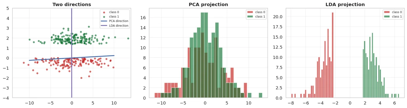
PCA took the most spread-out direction and the classes got MIXED. LDA took a direction with less spread, but the classes SEPARATED.

There's the difference. PCA chose the most spread-out direction and mixed up the classes. LDA found a direction with less spread that separates the classes.

python9 lines

from sklearn.model_selection import cross_val_score
from sklearn.pipeline import Pipeline
from sklearn.linear_model import LogisticRegression

print("Reduce to one component, then classify:")
for name, red in [("PCA(1)", PCA(n_components=1)), ("LDA(1)", LDA(n_components=1))]:
    b = cross_val_score(Pipeline([("sc", StandardScaler()), ("k", red),
                                  ("m", LogisticRegression())]), Xs_example, y_s, cv=5)
    print(f"  {name}: accuracy = {b.mean():.4f} ±{b.std():.4f}")

Output

Reduce to one component, then classify:
  PCA(1): accuracy = 0.8500 ±0.0506
  LDA(1): accuracy = 1.0000 ±0.0000

The two faces of LDA

LDA is confusing because it does two different jobs, in one sklearn class:

python8 lines

show(pd.DataFrame([
    {"Role": "1. Dimension reduction", "Method": "transform()",
     "What it does": "Projects onto the directions that separate the classes",
     "Compare it with": "PCA (Chapter 27)"},
    {"Role": "2. Classifier", "Method": "predict()",
     "What it does": "Predicts from the class centres",
     "Compare it with": "LogisticRegression (Chapter 16)"},
]))

Role	Method	What it does	Compare it with
1. Dimension reduction	transform()	Projects onto the directions that separate the classes	PCA (Chapter 27)
2. Classifier	predict()	Predicts from the class centres	LogisticRegression (Chapter 16)

python11 lines

df = pd.read_csv(DATA / "penguins.csv")
pnum = ["bill_length_mm", "bill_depth_mm", "flipper_length_mm", "body_mass_g"]
from sklearn.impute import SimpleImputer
Xp = SimpleImputer(strategy="median").fit_transform(df[pnum])
yp = df.species.values

l = LDA().fit(Xp, yp)
print("LDA does both jobs:")
print(f"  transform() -> {l.transform(Xp).shape}  (from 4 columns to {l.transform(Xp).shape[1]})")
print(f"  predict()   -> {l.predict(Xp[:5])}")
print(f"  score()     -> {l.score(Xp, yp):.4f}")

Output

LDA does both jobs:
  transform() -> (344, 2)  (from 4 columns to 2)
  predict()   -> ['Adelie' 'Adelie' 'Adelie' 'Adelie' 'Adelie']
  score()     -> 0.9855

LDA's number of components is LIMITED

In PCA, n_components can go up to the number of columns. LDA has a hard limit:

Penguins have 3 classes, so LDA gives at most 2 components, even with 4 columns.

In binary classification (our ijaraga_berildi_30k), LDA gives only 1 component. So it brings 7 columns down to one.

python14 lines

print("We check the limit:")
for n in [1, 2, 3]:
    try:
        LDA(n_components=n).fit(Xp, yp)
        print(f"  n_components={n}: worked")
    except Exception as e:
        print(f"  n_components={n}: {type(e).__name__} -> {str(e)[:66]}")
print()
y_bin = pd.read_csv(DATA / "uy_ijara.csv")["ijaraga_berildi_30k"]
Xb = SimpleImputer(strategy="median").fit_transform(
    pd.read_csv(DATA / "uy_ijara.csv")[["xonalar", "maydon_m2", "qavat", "qavatlar_soni",
                                        "metro_km", "mebel", "qurilgan_yil"]])
l_bin = LDA().fit(Xb, y_bin)
print(f"Binary target, 7 columns -> LDA gives {l_bin.transform(Xb).shape[1]} component")

Output

We check the limit:
  n_components=1: worked
  n_components=2: worked
  n_components=3: ValueError -> n_components cannot be larger than min(n_features, n_classes - 1).

Binary target, 7 columns -> LDA gives 1 component

PCA and LDA for visualisation

python12 lines

Xp_s = StandardScaler().fit_transform(Xp)
Zp = PCA(n_components=2).fit_transform(Xp_s)
Zl = LDA(n_components=2).fit(Xp_s, yp).transform(Xp_s)

figure, axes = plt.subplots(1, 2, figsize=(13.5, 5))
for Z, ax, name in [(Zp, axes[0], "PCA (didn't see y)"), (Zl, axes[1], "LDA (knew y)")]:
    for t, colour in zip(["Adelie", "Gentoo", "Chinstrap"], ["#1a73e8", "#137333", "#c5221f"]):
        m = yp == t
        ax.scatter(Z[m, 0], Z[m, 1], s=26, alpha=.7, color=colour, label=t)
    ax.set_xlabel("component 1"); ax.set_ylabel("component 2")
    ax.set_title(name, fontweight="bold"); ax.legend(fontsize=8); ax.grid(alpha=.3)
fig("lda_penguins.png", caption="Both brought 4 dimensions down to 2. In LDA the classes are tighter and more clearly separated, because that's exactly what it aimed for.")

Both brought 4 dimensions down to 2. In LDA the classes are tighter and more clearly separated, because that's exactly what it aimed for.

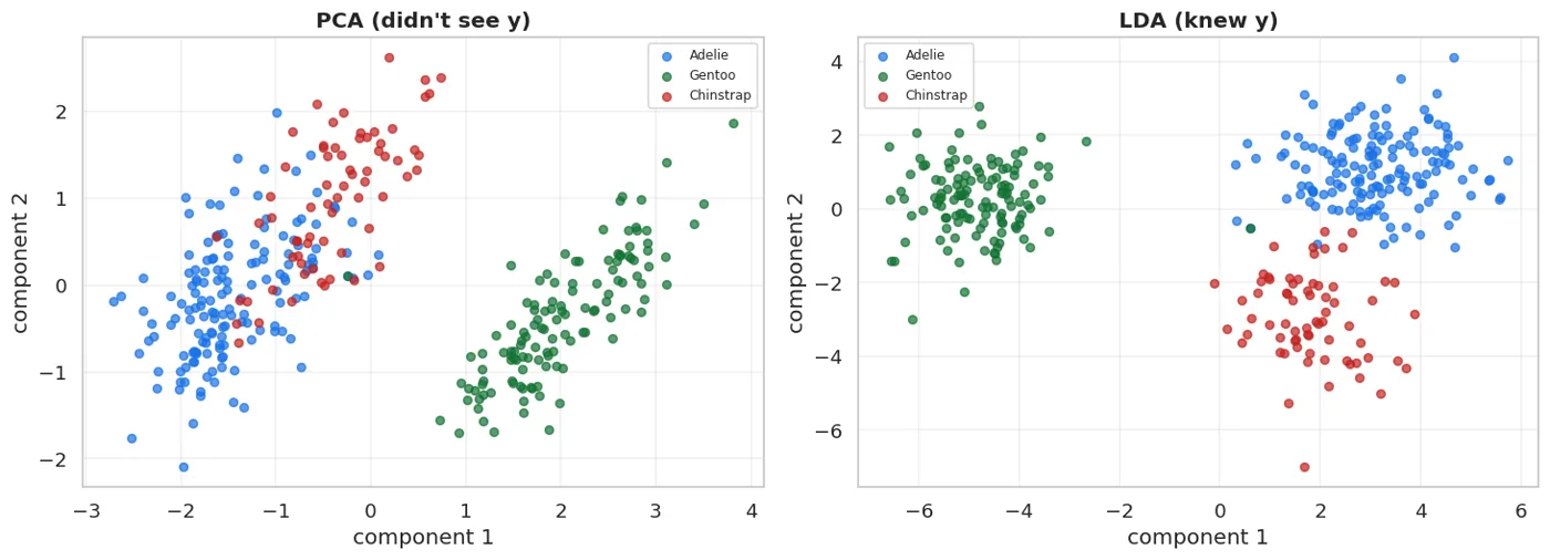
Both brought 4 dimensions down to 2. In LDA the classes are tighter and more clearly separated, because that's exactly what it aimed for.

LDA's pretty picture can fool you

On an LDA chart the classes always look better separated than on PCA. That's not an advantage of LDA: it was trained to do that.

If you compute the LDA projection on all the data and then use it to show how good a model is, that's leakage (Chapter 6). LDA has seen y.

So: you can use LDA for visualisation, but be careful about concluding "look how well the classes separate". It must be measured inside a Pipeline, with CV.

python9 lines

print("Proof: computing LDA on all the data vs inside the Pipeline:")
# WRONG: LDA on all the data
Z_bad = LDA(n_components=2).fit(Xp_s, yp).transform(Xp_s)
b_bad = cross_val_score(LogisticRegression(max_iter=2000), Z_bad, yp, cv=5)
# RIGHT: LDA inside the Pipeline
b_good = cross_val_score(Pipeline([("sc", StandardScaler()), ("l", LDA(n_components=2)),
                                   ("m", LogisticRegression(max_iter=2000))]), Xp, yp, cv=5)
print(f"  LDA on all the data (leakage) : {b_bad.mean():.4f} ±{b_bad.std():.4f}")
print(f"  LDA inside the Pipeline (right): {b_good.mean():.4f} ±{b_good.std():.4f}")

Output

Proof: computing LDA on all the data vs inside the Pipeline:
  LDA on all the data (leakage) : 0.9884 ±0.0109
  LDA inside the Pipeline (right): 0.9854 ±0.0131

LDA as a classifier

python19 lines

from sklearn.discriminant_analysis import QuadraticDiscriminantAnalysis as QDA
from sklearn.naive_bayes import GaussianNB
from sklearn.ensemble import RandomForestClassifier
import time

print(f"{'model':<34} {'CV accuracy':>13} {'±':>8} {'time':>8}")
print("-" * 68)
for name, m in [
    ("LDA", LDA()),
    ("QDA", QDA()),
    ("LogisticRegression (Chapter 16)", LogisticRegression(max_iter=3000)),
    ("GaussianNB (Chapter 21)", GaussianNB()),
    ("RandomForest (Chapter 19)", RandomForestClassifier(n_estimators=200, random_state=42)),
]:
    t0 = time.perf_counter()
    b = cross_val_score(Pipeline([("i", SimpleImputer(strategy="median")),
                                  ("sc", StandardScaler()), ("m", m)]), df[pnum], yp, cv=5)
    dt = time.perf_counter() - t0
    print(f"{name:<34} {b.mean():>13.4f} {b.std():>8.4f} {dt:>7.2f}s")

Output

model                                CV accuracy        ±     time
--------------------------------------------------------------------
LDA                                       0.9796   0.0150    0.02s
QDA                                       0.9825   0.0109    0.02s
LogisticRegression (Chapter 16)           0.9854   0.0131    0.02s
GaussianNB (Chapter 21)                   0.9651   0.0117    0.02s
RandomForest (Chapter 19)                 0.9709   0.0131    0.59s

The penguins dataset is easy (we saw that in Chapter 43), so every model scores high.

LDA, QDA and Naive Bayes: three members of one family

All three come from the same idea: model the distribution of each class, then apply Bayes' theorem. The difference is in the assumption about the distribution.

python8 lines

show(pd.DataFrame([
    {"Model": "GaussianNB", "Assumption": "Every feature is independent (diagonal covariance)",
     "Boundary": "Curved", "Number of parameters": "The fewest"},
    {"Model": "LDA", "Assumption": "Every class has the SAME covariance",
     "Boundary": "LINEAR", "Number of parameters": "Medium"},
    {"Model": "QDA", "Assumption": "Each class has its OWN covariance",
     "Boundary": "Quadratic (curved)", "Number of parameters": "The most"},
]))

Model	Assumption	Boundary	Number of parameters
GaussianNB	Every feature is independent (diagonal covariance)	Curved	The fewest
LDA	Every class has the SAME covariance	LINEAR	Medium
QDA	Each class has its OWN covariance	Quadratic (curved)	The most

python18 lines

# show the boundary shape, on two features
X2d = SimpleImputer(strategy="median").fit_transform(df[["bill_length_mm", "flipper_length_mm"]])
X2d = StandardScaler().fit_transform(X2d)

figure, axes = plt.subplots(1, 3, figsize=(16, 4.4))
xx, yy = np.meshgrid(np.linspace(X2d[:, 0].min()-.5, X2d[:, 0].max()+.5, 200),
                     np.linspace(X2d[:, 1].min()-.5, X2d[:, 1].max()+.5, 200))
grid = np.c_[xx.ravel(), yy.ravel()]
code = pd.Categorical(yp).codes
for ax, (name, m) in zip(axes, [("GaussianNB", GaussianNB()), ("LDA", LDA()), ("QDA", QDA())]):
    m.fit(X2d, code)
    Zg = m.predict(grid).reshape(xx.shape)
    ax.contourf(xx, yy, Zg, alpha=.22, cmap="viridis")
    ax.scatter(X2d[:, 0], X2d[:, 1], c=code, cmap="viridis", s=16, alpha=.8, edgecolors="k", linewidths=.2)
    ax.set_title(f"{name}  (accuracy {m.score(X2d, code):.3f})", fontweight="bold")
    ax.set_xlabel("bill_length"); ax.grid(alpha=.3)
axes[0].set_ylabel("flipper_length")
fig("lda_qda_chegara.png", caption="LDA's boundaries are straight lines. QDA draws curves, because each class is allowed its own covariance.")

LDA's boundaries are straight lines. QDA draws curves, because each class is allowed its own covariance.

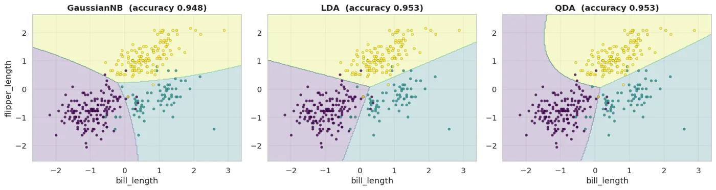
LDA's boundaries are straight lines. QDA draws curves, because each class is allowed its own covariance.

QDA doesn't fail on small data: it memorises SILENTLY

I had written this section as "QDA doesn't work on a small class; it raises a Singular matrix error". I measured it: that wasn't confirmed, and the truth is more dangerous.

QDA estimates a separate covariance matrix for each class. When a class has few rows it doesn't raise an error: it simply memorises those rows.

The table below shows it.

python22 lines

import warnings
from sklearn.model_selection import train_test_split

X2d_t = X2d
r3 = np.random.default_rng(0)
print(f"{'rows per class':>14} {'QDA train':>10} {'QDA test':>9} {'LDA test':>9} {'warnings':>9}")
print("-" * 56)
for n_s in [60, 20, 8, 4]:
    idx = []
    for cls in np.unique(code):
        m = np.where(code == cls)[0]
        idx.extend(r3.choice(m, min(n_s, len(m)), replace=False))
    idx = np.array(idx)
    Xk, yk = X2d_t[idx], code[idx]
    tr, te, ytr, yte = train_test_split(Xk, yk, test_size=.4, random_state=42, stratify=yk)
    with warnings.catch_warnings(record=True) as w:
        warnings.simplefilter("always")
        q = QDA().fit(tr, ytr)
        n_warn = len(w)
    lq = LDA().fit(tr, ytr)
    print(f"{n_s:>14} {q.score(tr, ytr):>10.3f} {q.score(te, yte):>9.3f} "
          f"{lq.score(te, yte):>9.3f} {n_warn:>9}")

Output

rows per class  QDA train  QDA test  LDA test  warnings
--------------------------------------------------------
            60      0.935     0.931     0.944         0
            20      0.917     0.917     0.958         0
             8      0.929     0.600     1.000         0
             4      0.286     0.400     1.000         2

Read the table row by row:

60 and 20 rows: QDA and LDA are almost the same, and train and test are close. All good.
8 rows: QDA scores 0.929 on train and 0.600 on test. In other words, it memorised. And notice: zero warnings. Nothing tells you you're making a mistake.
4 rows: QDA breaks completely (train 0.286, worse than chance), and only here does it raise a warning.

LDA stays stable in every case, because it estimates one shared covariance matrix, which means it uses the rows of all the classes together.

No error does NOT mean "it's working correctly"

This is a recurring theme of the book. In Chapter 1, leakage raised no error. In Chapter 6, StandardScaler fitted on all the data raised no error. Here, QDA on a small class raised no error.

In all three, the code runs, a number comes out, and it's a lie.

There's one defence: look at the train and test scores side by side. In the table above, the 8-row line has a gap of 0.33, which jumps out immediately. If you only look at the test score, you notice nothing.

The rule: unless each class has at least 10 times as many rows as there are columns, don't use QDA. Take LDA or GaussianNB.

When to choose LDA

python8 lines

show(pd.DataFrame([
    {"Situation": "Visualisation, seeing how the classes separate", "Choice": "LDA transform (but watch out for leakage)"},
    {"Situation": "Many columns, few classes", "Choice": "LDA: reduces to n_classes-1 dimensions"},
    {"Situation": "You need a fast, simple classifier", "Choice": "LDA: no parameters, nothing to tune"},
    {"Situation": "A non-linear boundary", "Choice": "QDA or a tree (Chapter 18)"},
    {"Situation": "Little data", "Choice": "LDA (not QDA)"},
    {"Situation": "You need probabilities", "Choice": "Both LDA and LogisticRegression give them"},
]))

Situation	Choice
Visualisation, seeing how the classes separate	LDA transform (but watch out for leakage)
Many columns, few classes	LDA: reduces to n_classes-1 dimensions
You need a fast, simple classifier	LDA: no parameters, nothing to tune
A non-linear boundary	QDA or a tree (Chapter 18)
Little data	LDA (not QDA)
You need probabilities	Both LDA and LogisticRegression give them

An advantage of LDA that's rarely mentioned

LDA has no parameters to tune. No alpha, C, max_depth or n_estimators.

So it doesn't need the GridSearchCV from Chapter 24. That makes it very handy as a fast baseline model: one line, a result, and then you check whether more complex models beat it.

Add it to the baseline sequence from Chapter 7: DummyClassifier -> LDA -> LogisticRegression -> complex models.

PCA and LDA side by side

python8 lines

show(pd.DataFrame([
    {"": "PCA", "Sees y?": "NO (unsupervised)",
     "What it maximises": "Variance", "Component limit": "up to n_features",
     "Leakage risk": "None (doesn't use y)"},
    {"": "LDA", "Sees y?": "YES (supervised)",
     "What it maximises": "Class separation", "Component limit": "n_classes - 1",
     "Leakage risk": "YES: it must be used inside a Pipeline"},
]))

	Sees y?	What it maximises	Component limit	Leakage risk
PCA	NO (unsupervised)	Variance	up to n_features	None (doesn't use y)
LDA	YES (supervised)	Class separation	n_classes - 1	YES: it must be used inside a Pipeline

python16 lines

print("We compare the two on our binary data:")
Xd = pd.read_csv(DATA / "uy_ijara.csv")
numd = ["xonalar", "maydon_m2", "qavat", "qavatlar_soni", "metro_km", "mebel", "qurilgan_yil"]
Xf, yf = Xd[numd], Xd["ijaraga_berildi_30k"]
print(f"{'variant':<40} {'CV F1':>9} {'±':>8}")
print("-" * 60)
for name, steps in [
    ("NO reduction (7 columns)", [("i", SimpleImputer(strategy="median")), ("sc", StandardScaler()),
                                  ("m", LogisticRegression(max_iter=3000))]),
    ("PCA(2)", [("i", SimpleImputer(strategy="median")), ("sc", StandardScaler()),
                ("k", PCA(n_components=2)), ("m", LogisticRegression(max_iter=3000))]),
    ("LDA(1): the maximum for binary", [("i", SimpleImputer(strategy="median")), ("sc", StandardScaler()),
                                        ("k", LDA(n_components=1)), ("m", LogisticRegression(max_iter=3000))]),
]:
    b = cross_val_score(Pipeline(steps), Xf, yf, cv=5, scoring="f1")
    print(f"{name:<40} {b.mean():>9.4f} {b.std():>8.4f}")

Output

We compare the two on our binary data:
variant                                      CV F1        ±
------------------------------------------------------------
NO reduction (7 columns)                    0.7219   0.0106
PCA(2)                                      0.7302   0.0091
LDA(1): the maximum for binary              0.7245   0.0101

What we learned today

python9 lines

show(pd.DataFrame([
    {"Concept": "PCA vs LDA", "In one sentence": "PCA maximises variance, LDA maximises class separation"},
    {"Concept": "LDA's two faces", "In one sentence": "transform() reduces, predict() classifies"},
    {"Concept": "The component limit", "In one sentence": "n_classes - 1; only 1 for binary"},
    {"Concept": "Leakage risk", "In one sentence": "LDA sees y: it MUST be used inside a Pipeline"},
    {"Concept": "LDA / QDA / GaussianNB", "In one sentence": "One family; they differ in the covariance assumption"},
    {"Concept": "QDA's limitation", "In one sentence": "Fails when each class has few rows"},
    {"Concept": "LDA's advantage", "In one sentence": "NO parameters to tune: a fast baseline model"},
]))

Concept	In one sentence
PCA vs LDA	PCA maximises variance, LDA maximises class separation
LDA's two faces	transform() reduces, predict() classifies
The component limit	n_classes - 1; only 1 for binary
Leakage risk	LDA sees y: it MUST be used inside a Pipeline
LDA / QDA / GaussianNB	One family; they differ in the covariance assumption
QDA's limitation	Fails when each class has few rows
LDA's advantage	NO parameters to tune: a fast baseline model

That completes Part 6. You now know how to work with unlabelled data: reducing dimensions (27), grouping (28), and reduction that takes the target into account (29).

The next part is deep learning.

previous28. Clustering: K-Means, DBSCAN, hierarchical next30. Neural network basics

Questions about this chapter?

The course, homework review and the other five books are in Uzbek. Questions in English are welcome on Telegram.

Write on Telegram Contents