Backpropagation and optimizers
The scene: the "backward" part of Chapter 30
In Chapter 30 we trained a network. The code had lines like these:
dz1 = da1 * (z1 > 0)        # the ReLU derivative
dW1 = X.T @ dz1
That is backpropagation. And it's not magic: it's the chain rule from secondary school.
This chapter opens it up, then looks at the methods that speed up training.
The chain rule: one example
At school you were taught: if
A neural network is a long chain of functions. So its gradient is a chain of products too.
import numpy as np
import pandas as pd

# the simplest chain: x -> z1 = w1*x -> a1 = z1^2 -> z2 = w2*a1 -> L = (z2 - y)^2
x, y_true, w1, w2 = 2.0, 10.0, 3.0, 0.5

# FORWARD
z1 = w1 * x
a1 = z1 ** 2
z2 = w2 * a1
L = (z2 - y_true) ** 2
print(f"FORWARD: x={x} -> z1={z1} -> a1={a1} -> z2={z2} -> L={L}")
print()

# BACKWARD, by the chain rule
dL_dz2 = 2 * (z2 - y_true)
dz2_dw2 = a1
dz2_da1 = w2
da1_dz1 = 2 * z1
dz1_dw1 = x

dL_dw2 = dL_dz2 * dz2_dw2
dL_dw1 = dL_dz2 * dz2_da1 * da1_dz1 * dz1_dw1

print("BACKWARD (the chain rule):")
print(f"  dL/dz2 = 2*(z2-y)        = {dL_dz2}")
print(f"  dL/dw2 = dL/dz2 * a1     = {dL_dw2}")
print(f"  dL/dw1 = dL/dz2 * w2 * 2*z1 * x = {dL_dw1}")
FORWARD: x=2.0 -> z1=6.0 -> a1=36.0 -> z2=18.0 -> L=64.0

BACKWARD (the chain rule):
  dL/dz2 = 2*(z2-y)        = 16.0
  dL/dw2 = dL/dz2 * a1     = 576.0
  dL/dw1 = dL/dz2 * w2 * 2*z1 * x = 192.0
A check: you can also compute the gradient numerically. That's the classic way to check backpropagation.
def loss(w1_, w2_):
    return (w2_ * (w1_ * x) ** 2 - y_true) ** 2

h = 1e-6
numeric_w1 = (loss(w1 + h, w2) - loss(w1 - h, w2)) / (2 * h)
numeric_w2 = (loss(w1, w2 + h) - loss(w1, w2 - h)) / (2 * h)

print(f"{'parameter':>10} {'analytic':>14} {'numeric':>14} {'difference':>12}")
print("-" * 54)
print(f"{'w1':>10} {dL_dw1:>14.6f} {numeric_w1:>14.6f} {abs(dL_dw1-numeric_w1):>12.2e}")
print(f"{'w2':>10} {dL_dw2:>14.6f} {numeric_w2:>14.6f} {abs(dL_dw2-numeric_w2):>12.2e}")
 parameter       analytic        numeric   difference
------------------------------------------------------
        w1     192.000000     192.000000     2.68e-08
        w2     576.000000     576.000000     4.75e-09
Gradient checking: a way to test your own code
If you write backpropagation by hand, check it this way: the analytic gradient must match the numeric one.
If the difference is bigger than 1e-6, your code has a bug.
This used to be mandatory before torch and tensorflow existed. Today there's automatic differentiation (Chapter 33), but the skill of checking is still useful.
The vanishing gradient: sigmoid's punishment
We said in Chapter 30: where the sigmoid is flat, its derivative is close to zero. In a deep network that effect multiplies.
def sigmoid(z):
    return 1 / (1 + np.exp(-np.clip(z, -500, 500)))

print("In the chain rule the derivatives are MULTIPLIED.")
print("The sigmoid derivative's maximum is 0.25 (at z=0):")
print()
print(f"{'layers':>10} {'sigmoid (0.25^n)':>20} {'ReLU (1^n)':>14}")
print("-" * 48)
for n in [1, 3, 5, 10, 20]:
    print(f"{n:>10} {0.25**n:>20.2e} {1.0**n:>14.1f}")
In the chain rule the derivatives are MULTIPLIED.
The sigmoid derivative's maximum is 0.25 (at z=0):

    layers     sigmoid (0.25^n)     ReLU (1^n)
------------------------------------------------
         1             2.50e-01            1.0
         3             1.56e-02            1.0
         5             9.77e-04            1.0
        10             9.54e-07            1.0
        20             9.09e-13            1.0
In a 20-layer sigmoid network the gradient drops to 9e-13, which means the first layer doesn't learn at all.
With ReLU the derivative is exactly 1 on the positive side, so the gradient doesn't weaken. That's why ReLU was a revolution.
import matplotlib.pyplot as plt

# measure it in practice: the gradient's size in a deep network
def measure_gradient(n_layers, activation="sigmoid", seed=42):
    r = np.random.default_rng(seed)
    X = r.normal(size=(200, 20))
    W = [r.normal(0, 1 / np.sqrt(20), (20, 20)) for _ in range(n_layers)]
    a = X
    states = [a]
    for Wi in W:
        z = a @ Wi
        a = sigmoid(z) if activation == "sigmoid" else np.maximum(0, z)
        states.append(a)
    # backward: track the gradient's size starting from the last layer
    g = np.ones_like(a)
    sizes = []
    for i in range(n_layers - 1, -1, -1):
        if activation == "sigmoid":
            g = g * states[i + 1] * (1 - states[i + 1])
        else:
            g = g * (states[i + 1] > 0)
        g = g @ W[i].T
        sizes.append(float(np.abs(g).mean()))
    return sizes[::-1]

sig_g = measure_gradient(12, "sigmoid")
relu_g = measure_gradient(12, "relu")

figure, ax = plt.subplots(figsize=(9.5, 4.6))
ax.semilogy(range(1, 13), sig_g, "o-", lw=2, label="sigmoid", color="#c5221f")
ax.semilogy(range(1, 13), relu_g, "o-", lw=2, label="ReLU", color="#137333")
ax.set_xlabel("Layer (1 = closest to the input)")
ax.set_ylabel("Mean gradient size (log scale)")
ax.set_title("The vanishing gradient, in a 12-layer network", fontweight="bold")
ax.legend(); ax.grid(alpha=.3, which="both")
fig("gradient_yoqolishi.png", caption="With sigmoid the gradient doesn't reach the first layers. With ReLU it survives.")

print(f"{'layer':>8} {'sigmoid gradient':>20} {'ReLU gradient':>16}")
print("-" * 48)
for i in [0, 3, 7, 11]:
    print(f"{i+1:>8} {sig_g[i]:>20.3e} {relu_g[i]:>16.3e}")
print()
print(f"At layer 1 the ratio: ReLU / sigmoid = {relu_g[0]/sig_g[0]:.0f} times")
   layer     sigmoid gradient    ReLU gradient
------------------------------------------------
       1            2.317e-08        1.691e-02
       4            2.793e-06        4.642e-02
       8            8.294e-04        2.057e-01
      12            2.429e-01        8.786e-01

At layer 1 the ratio: ReLU / sigmoid = 729616 times
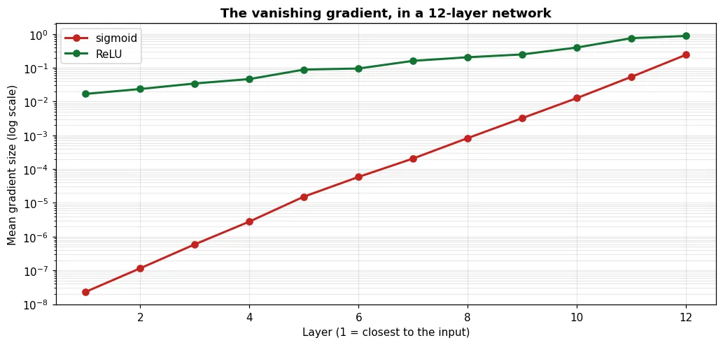
With sigmoid the gradient doesn't reach the first layers. With ReLU it survives.
Weight initialization
Can you start the weights at zero? No, and the reason is simple.
print("If every weight is ZERO:")
W_zero = np.zeros((4, 3))
X_t = np.random.default_rng(0).normal(size=(5, 4))
print(f"  output: {np.unique(np.round(X_t @ W_zero, 6))}  -> every neuron is THE SAME")
print("  Every neuron gets the same gradient and changes the same way.")
print("  So a 100-neuron layer equals 1 neuron: the SYMMETRY never breaks.")
print()
print("If the weights are very LARGE:")
r = np.random.default_rng(42)
for std in [0.01, 1.0, 10.0]:
    a = r.normal(size=(500, 50))
    for _ in range(5):
        a = np.tanh(a @ r.normal(0, std, (50, 50)))
    print(f"  std={std:<6} after 5 layers, output |mean| = {np.abs(a).mean():.6f}")
If every weight is ZERO:
  output: [0.]  -> every neuron is THE SAME
  Every neuron gets the same gradient and changes the same way.
  So a 100-neuron layer equals 1 neuron: the SYMMETRY never breaks.

If the weights are very LARGE:
  std=0.01   after 5 layers, output |mean| = 0.000001
  std=1.0    after 5 layers, output |mean| = 0.915228
  std=10.0   after 5 layers, output |mean| = 0.992363
Too small, and the signal dies. Too large, and it saturates (with tanh it sticks to ±1).
The fix: an initialization adjusted to the layer's size.
show(pd.DataFrame([
    {"Method": "Xavier / Glorot", "Formula": "std = sqrt(2 / (n_in + n_out))",
     "When": "tanh, sigmoid", "In Keras": "glorot_uniform (THE DEFAULT)"},
    {"Method": "He / Kaiming", "Formula": "std = sqrt(2 / n_in)",
     "When": "ReLU and its variants", "In Keras": "he_normal"},
    {"Method": "Zero", "Formula": "0", "When": "ONLY for the bias", "In Keras": "zeros"},
]))
| Method | Formula | When | In Keras |
|---|---|---|---|
| Xavier / Glorot | std = sqrt(2 / (n_in + n_out)) | tanh, sigmoid | glorot_uniform (THE DEFAULT) |
| He / Kaiming | std = sqrt(2 / n_in) | ReLU and its variants | he_normal |
| Zero | 0 | ONLY for the bias | zeros |
print("He and Xavier in practice: how well the signal survives in a 10-layer ReLU network:")
print(f"{'initialization':<22} {'|output| after 10 layers':>30}")
print("-" * 54)
n = 100
for name, std in [("very small (0.01)", 0.01), ("Xavier (sqrt(1/n))", np.sqrt(1/n)),
                  ("He (sqrt(2/n))", np.sqrt(2/n)), ("very large (0.5)", 0.5)]:
    a = r.normal(size=(300, n))
    for _ in range(10):
        a = np.maximum(0, a @ r.normal(0, std, (n, n)))
    print(f"{name:<22} {np.abs(a).mean():>30.6f}")
He and Xavier in practice: how well the signal survives in a 10-layer ReLU network:
initialization               |output| after 10 layers
------------------------------------------------------
very small (0.01)                            0.000000
Xavier (sqrt(1/n))                           0.016119
He (sqrt(2/n))                               0.597205
very large (0.5)                        120407.435643
He initialization keeps the signal stable for ReLU, which is why it's the standard in ReLU networks.
Optimizers: the descendants of gradient descent
In Chapter 13 we saw the simplest rule:
In practice there are better methods.
show(pd.DataFrame([
    {"Optimizer": "SGD", "Idea": "Plain gradient descent",
     "Strength": "Simple, little memory", "Weakness": "Slow, the learning rate is delicate"},
    {"Optimizer": "SGD + Momentum", "Idea": "Keeps the previous direction as a 'velocity'",
     "Strength": "Reduces oscillation", "Weakness": "One more parameter"},
    {"Optimizer": "RMSProp", "Idea": "Each parameter gets its own learning rate",
     "Strength": "Adapts to different scales", "Weakness": "No momentum"},
    {"Optimizer": "Adam", "Idea": "Momentum + RMSProp together",
     "Strength": "THE DEFAULT CHOICE: works in most cases", "Weakness": "More memory"},
    {"Optimizer": "AdamW", "Idea": "Adam + correct weight decay",
     "Strength": "The standard for Transformers", "Weakness": "-"},
]))
| Optimizer | Idea | Strength | Weakness |
|---|---|---|---|
| SGD | Plain gradient descent | Simple, little memory | Slow, the learning rate is delicate |
| SGD + Momentum | Keeps the previous direction as a 'velocity' | Reduces oscillation | One more parameter |
| RMSProp | Each parameter gets its own learning rate | Adapts to different scales | No momentum |
| Adam | Momentum + RMSProp together | THE DEFAULT CHOICE: works in most cases | More memory |
| AdamW | Adam + correct weight decay | The standard for Transformers | - |
Let me show the momentum idea, with a physical analogy: a ball rolling down a hill picks up speed.
def optimize(grad_f, start, alpha=0.1, steps=60, method="sgd", beta=0.9):
    w = np.array(start, dtype=float)
    v = np.zeros_like(w)
    s = np.zeros_like(w)
    path = [w.copy()]
    for k in range(1, steps + 1):
        g = grad_f(w)
        if method == "sgd":
            w = w - alpha * g
        elif method == "momentum":
            v = beta * v + (1 - beta) * g
            w = w - alpha * v / (1 - beta ** k)
        elif method == "adam":
            v = 0.9 * v + 0.1 * g
            s = 0.999 * s + 0.001 * g ** 2
            v_t = v / (1 - 0.9 ** k)
            s_t = s / (1 - 0.999 ** k)
            w = w - alpha * v_t / (np.sqrt(s_t) + 1e-8)
        path.append(w.copy())
    return np.array(path)

# a "stretched bowl": steep along one axis, flat along the other
def grad_stretched(w):
    return np.array([20 * w[0], 1 * w[1]])

paths = {u: optimize(grad_stretched, [-4.0, -4.0], alpha=0.08, method=u)
         for u in ["sgd", "momentum", "adam"]}

figure, ax = plt.subplots(figsize=(9.5, 5))
xx, yy = np.meshgrid(np.linspace(-5, 2, 200), np.linspace(-5, 2, 200))
ax.contour(xx, yy, 10 * xx**2 + 0.5 * yy**2, levels=22, alpha=.3, colors="gray")
for (name, path), colour in zip(paths.items(), ["#c5221f", "#f9ab00", "#137333"]):
    ax.plot(path[:, 0], path[:, 1], "o-", ms=3, lw=1.5, label=name, color=colour, alpha=.85)
ax.plot(0, 0, "k*", ms=16, label="target")
ax.legend(); ax.set_title("Three optimizers in a stretched bowl", fontweight="bold")
ax.grid(alpha=.3)
fig("optimizerlar.png", caption="SGD zigzags. Momentum is smoother. Adam adapts its step to each axis.")

print(f"{'optimizer':<12} {'distance after 60 steps':>26}")
print("-" * 40)
for name, path in paths.items():
    print(f"{name:<12} {np.linalg.norm(path[-1]):>26.6f}")
optimizer       distance after 60 steps
----------------------------------------
sgd                            0.026874
momentum                       0.055361
adam                           0.548182
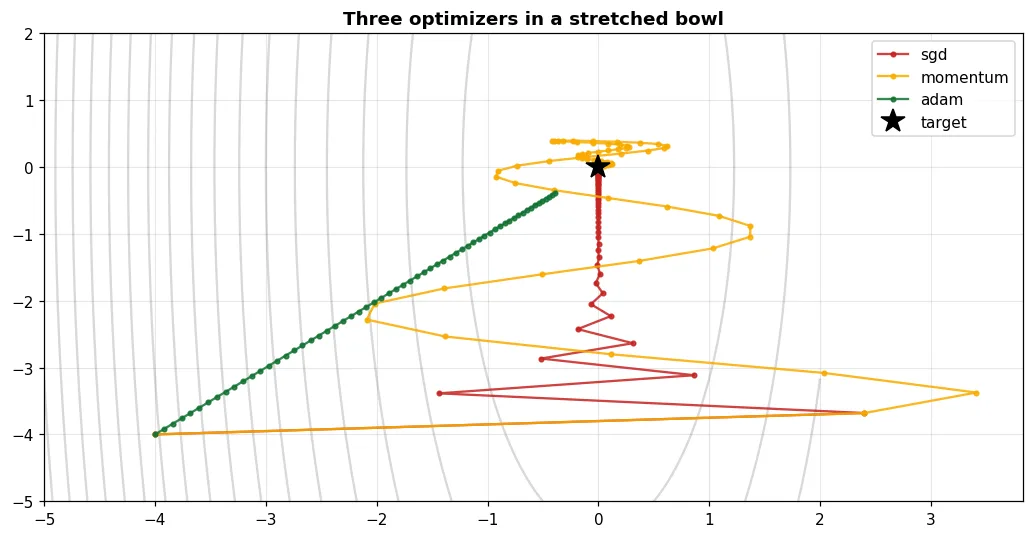
SGD zigzags. Momentum is smoother. Adam adapts its step to each axis.
In practice: comparing optimizers
Column names
The rental data has Uzbek column names. xonalar rooms, maydon_m2 area in m², qavat floor, qavatlar_soni floors in the building, metro_km distance to the metro, mebel furnished (0/1), qurilgan_yil year built. The target ijaraga_berildi_30k means rented within 30 days.
import os
os.environ.setdefault("CUDA_VISIBLE_DEVICES", "-1")   # CPU, for reproducibility
import torch
import torch.nn as nn
torch.manual_seed(42)
torch.set_num_threads(2)

from sklearn.model_selection import train_test_split
from sklearn.preprocessing import StandardScaler
from sklearn.impute import SimpleImputer

df = pd.read_csv(DATA / "uy_ijara.csv")
num = ["xonalar", "maydon_m2", "qavat", "qavatlar_soni", "metro_km", "mebel", "qurilgan_yil"]
Xd = SimpleImputer(strategy="median").fit_transform(df[num])
yd = df["ijaraga_berildi_30k"].to_numpy(dtype=np.float32)
X_tr, X_te, y_tr, y_te = train_test_split(Xd, yd, test_size=0.3, random_state=42, stratify=yd)
sc = StandardScaler().fit(X_tr)
Xt = torch.tensor(sc.transform(X_tr), dtype=torch.float32)
Yt = torch.tensor(y_tr).unsqueeze(1)
Xv = torch.tensor(sc.transform(X_te), dtype=torch.float32)
Yv = torch.tensor(y_te).unsqueeze(1)

def train(opt_name, epochs=120, lr=0.01):
    torch.manual_seed(42)
    model = nn.Sequential(nn.Linear(Xt.shape[1], 16), nn.ReLU(), nn.Linear(16, 1))
    criterion = nn.BCEWithLogitsLoss()
    opt = {"SGD": torch.optim.SGD(model.parameters(), lr=lr),
           "SGD+Momentum": torch.optim.SGD(model.parameters(), lr=lr, momentum=0.9),
           "RMSProp": torch.optim.RMSprop(model.parameters(), lr=lr),
           "Adam": torch.optim.Adam(model.parameters(), lr=lr)}[opt_name]
    history = []
    for _ in range(epochs):
        opt.zero_grad()
        loss = criterion(model(Xt), Yt)
        loss.backward()
        opt.step()
        history.append(float(loss))
    with torch.no_grad():
        val = float(criterion(model(Xv), Yv))
        acc = float(((torch.sigmoid(model(Xv)) > .5).float() == Yv).float().mean())
    return history, val, acc

print(f"{'optimizer':<16} {'train loss':>17} {'val loss':>15} {'val accuracy':>13}")
print("-" * 66)
histories = {}
for name in ["SGD", "SGD+Momentum", "RMSProp", "Adam"]:
    tr, val, acc = train(name)
    histories[name] = tr
    print(f"{name:<16} {tr[-1]:>17.4f} {val:>15.4f} {acc:>13.4f}")
optimizer               train loss        val loss  val accuracy
------------------------------------------------------------------
SGD                         0.6855          0.6862        0.5583
SGD+Momentum                0.5794          0.5214        0.7861
RMSProp                     0.5237          0.5020        0.7667
Adam                        0.5460          0.4952        0.7722
figure, ax = plt.subplots(figsize=(9.5, 4.6))
for (name, tr), colour in zip(histories.items(), ["#c5221f", "#f9ab00", "#1a73e8", "#137333"]):
    ax.plot(tr, lw=2, label=name, color=colour)
ax.set_xlabel("Epoch"); ax.set_ylabel("Train loss")
ax.set_title("The same network, four optimizers", fontweight="bold")
ax.legend(); ax.grid(alpha=.3)
fig("optimizer_tarix.png", caption="Adam and RMSProp drop faster. Plain SGD is slower, but in the end they all converge.")
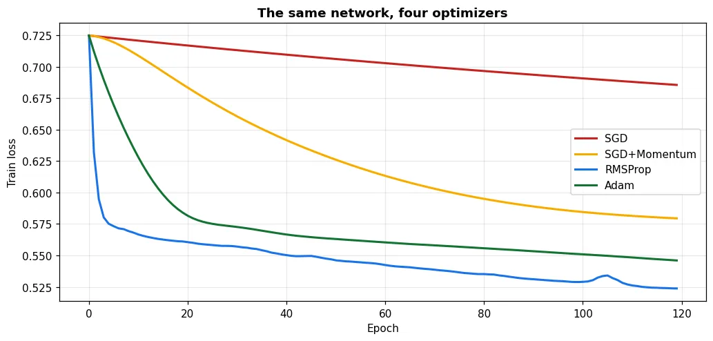
Adam and RMSProp drop faster. Plain SGD is slower, but in the end they all converge.
The practical choice
Start with Adam, with lr=0.001 (the default in Keras and PyTorch).
If the result is unsatisfying:
- lower or raise lr by 3 times (0.0003 or 0.003)
- if you're training a Transformer: AdamW
- with a very large network and very much data, SGD + momentum sometimes generalises better
Switching optimizers is one of the last options. First you check the architecture and the data (Chapter 11).
The learning-rate schedule
epochs = 100
schedules = {
    "constant": np.full(epochs, 0.01),
    "step (/10 every 30)": 0.01 * (0.1 ** (np.arange(epochs) // 30)),
    "exponential": 0.01 * 0.97 ** np.arange(epochs),
    "cosine": 0.01 * (1 + np.cos(np.pi * np.arange(epochs) / epochs)) / 2,
}
figure, ax = plt.subplots(figsize=(9.5, 4.2))
for name, j in schedules.items():
    ax.plot(j, lw=2, label=name)
ax.set_xlabel("Epoch"); ax.set_ylabel("Learning rate")
ax.set_title("Learning-rate schedules", fontweight="bold")
ax.legend(); ax.grid(alpha=.3)
fig("lr_jadval.png", caption="Big steps at the start (fast learning), small steps at the end (fine tuning).")
print("The idea: move fast at the start, adjust carefully at the end.")
The idea: move fast at the start, adjust carefully at the end.
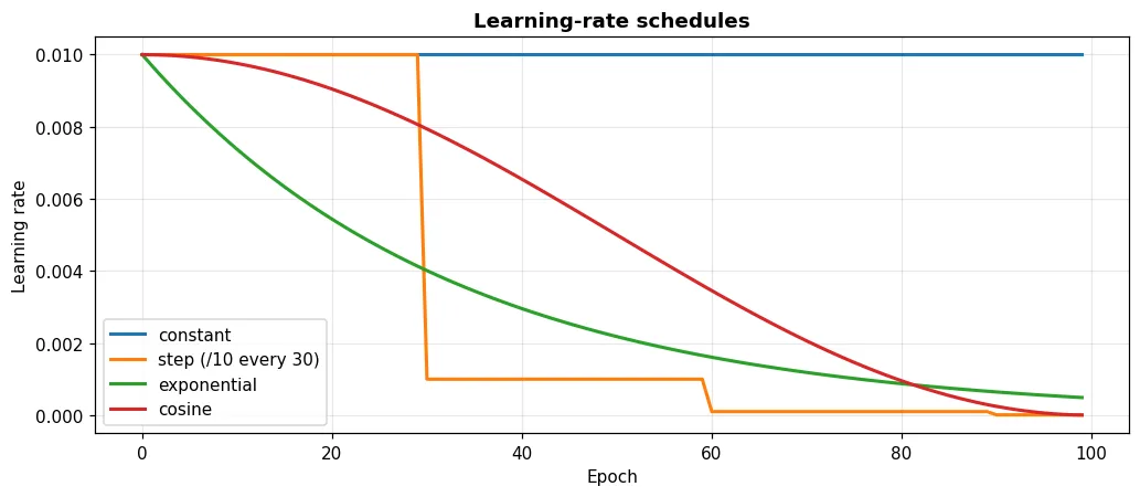
Big steps at the start (fast learning), small steps at the end (fine tuning).
def train_schedule(sched_name, epochs=150):
    torch.manual_seed(42)
    model = nn.Sequential(nn.Linear(Xt.shape[1], 16), nn.ReLU(), nn.Linear(16, 1))
    opt = torch.optim.SGD(model.parameters(), lr=0.05, momentum=0.9)
    sched = {"none": None,
             "StepLR": torch.optim.lr_scheduler.StepLR(opt, step_size=50, gamma=0.1),
             "CosineAnnealing": torch.optim.lr_scheduler.CosineAnnealingLR(opt, T_max=epochs)}[sched_name]
    criterion = nn.BCEWithLogitsLoss()
    for _ in range(epochs):
        opt.zero_grad(); loss = criterion(model(Xt), Yt); loss.backward(); opt.step()
        if sched: sched.step()
    with torch.no_grad():
        return float(criterion(model(Xv), Yv)), float(((torch.sigmoid(model(Xv)) > .5).float() == Yv).float().mean())

print(f"{'schedule':<20} {'val loss':>15} {'val accuracy':>13}")
print("-" * 52)
for name in ["none", "StepLR", "CosineAnnealing"]:
    v, a = train_schedule(name)
    print(f"{name:<20} {v:>15.4f} {a:>13.4f}")
schedule                    val loss  val accuracy
----------------------------------------------------
none                          0.5028        0.7694
StepLR                        0.5024        0.7722
CosineAnnealing               0.5049        0.7694
Batch Normalization and Dropout
show(pd.DataFrame([
    {"Method": "BatchNorm", "What it does": "Normalises each layer's output",
     "Benefit": "Faster training, allows a larger lr", "Where": "AFTER Linear/Conv"},
    {"Method": "Dropout", "What it does": "Randomly switches off part of the neurons during training",
     "Benefit": "Reduces overfitting", "Where": "After the hidden layers"},
]))
| Method | What it does | Benefit | Where |
|---|---|---|---|
| BatchNorm | Normalises each layer's output | Faster training, allows a larger lr | AFTER Linear/Conv |
| Dropout | Randomly switches off part of the neurons during training | Reduces overfitting | After the hidden layers |
def train_arch(name, epochs=200):
    torch.manual_seed(42)
    n = Xt.shape[1]
    model = {
        "plain": nn.Sequential(nn.Linear(n, 64), nn.ReLU(), nn.Linear(64, 32), nn.ReLU(), nn.Linear(32, 1)),
        "+ BatchNorm": nn.Sequential(nn.Linear(n, 64), nn.BatchNorm1d(64), nn.ReLU(),
                                     nn.Linear(64, 32), nn.BatchNorm1d(32), nn.ReLU(), nn.Linear(32, 1)),
        "+ Dropout(0.3)": nn.Sequential(nn.Linear(n, 64), nn.ReLU(), nn.Dropout(0.3),
                                        nn.Linear(64, 32), nn.ReLU(), nn.Dropout(0.3), nn.Linear(32, 1)),
    }[name]
    opt = torch.optim.Adam(model.parameters(), lr=0.01)
    criterion = nn.BCEWithLogitsLoss()
    for _ in range(epochs):
        model.train()
        opt.zero_grad(); loss = criterion(model(Xt), Yt); loss.backward(); opt.step()
    model.eval()
    with torch.no_grad():
        tr_l = float(criterion(model(Xt), Yt))
        va_l = float(criterion(model(Xv), Yv))
        acc = float(((torch.sigmoid(model(Xv)) > .5).float() == Yv).float().mean())
    return tr_l, va_l, acc

print(f"{'architecture':<18} {'train loss':>12} {'val loss':>11} {'gap':>8} {'val accuracy':>13}")
print("-" * 68)
for name in ["plain", "+ BatchNorm", "+ Dropout(0.3)"]:
    tr_l, va_l, acc = train_arch(name)
    print(f"{name:<18} {tr_l:>12.4f} {va_l:>11.4f} {va_l-tr_l:>8.4f} {acc:>13.4f}")
architecture         train loss    val loss      gap  val accuracy
--------------------------------------------------------------------
plain                    0.1152      1.2849   1.1697        0.6472
+ BatchNorm              0.1498      0.9738   0.8240        0.6500
+ Dropout(0.3)           0.4290      0.5522   0.1232        0.7333
The "gap" column is a measure of overfitting (the train/test gap from Chapter 2). Dropout is expected to shrink it.
Dropout must be SWITCHED OFF in eval() mode
In PyTorch the difference between model.train() and model.eval() is vital:
train(): Dropout switches neurons off, BatchNorm uses the batch statisticseval(): Dropout turns off, BatchNorm uses the stored statistics
If you don't call eval(), your predictions are different every time you call the model, because Dropout works at random.
This is the most common mistake in PyTorch. In Keras it's automatic.
torch.manual_seed(0)
m_drop = nn.Sequential(nn.Linear(Xt.shape[1], 16), nn.ReLU(), nn.Dropout(0.5), nn.Linear(16, 1))
m_drop.train()
with torch.no_grad():
    three_train = [float(m_drop(Xv[:1])) for _ in range(3)]
m_drop.eval()
with torch.no_grad():
    three_eval = [float(m_drop(Xv[:1])) for _ in range(3)]
print(f"3 times in train() mode: {[round(v, 4) for v in three_train]}  <-- ALL DIFFERENT")
print(f"3 times in eval()  mode: {[round(v, 4) for v in three_eval]}  <-- the same")
3 times in train() mode: [-0.113, -0.1975, -0.7742]  <-- ALL DIFFERENT
3 times in eval()  mode: [-0.4892, -0.4892, -0.4892]  <-- the same
What we learned today
show(pd.DataFrame([
    {"Concept": "Backpropagation", "In one sentence": "The chain rule: not magic"},
    {"Concept": "Gradient checking", "In one sentence": "The analytic and numeric gradients must match"},
    {"Concept": "The vanishing gradient", "In one sentence": "The sigmoid derivative's max is 0.25: 9e-13 after 20 layers"},
    {"Concept": "Weight initialization", "In one sentence": "Never zero (symmetry); He for ReLU"},
    {"Concept": "Adam", "In one sentence": "Momentum + RMSProp; the default choice, lr=0.001"},
    {"Concept": "LR schedule", "In one sentence": "Big steps at the start, small ones at the end"},
    {"Concept": "BatchNorm", "In one sentence": "Faster training, a larger lr"},
    {"Concept": "Dropout", "In one sentence": "Against overfitting; it turns off in eval()"},
]))
| Concept | In one sentence |
|---|---|
| Backpropagation | The chain rule: not magic |
| Gradient checking | The analytic and numeric gradients must match |
| The vanishing gradient | The sigmoid derivative's max is 0.25: 9e-13 after 20 layers |
| Weight initialization | Never zero (symmetry); He for ReLU |
| Adam | Momentum + RMSProp; the default choice, lr=0.001 |
| LR schedule | Big steps at the start, small ones at the end |
| BatchNorm | Faster training, a larger lr |
| Dropout | Against overfitting; it turns off in eval() |
Next chapter: we put these ideas into practice with Keras, with far less code.
Questions about this chapter?
The course, homework review and the other five books are in Uzbek. Questions in English are welcome on Telegram.