CNN: convolutional neural networks
The scene: why an ordinary network isn't enough for images
In Chapters 30-33 the networks didn't beat simple models on tabular data. We measured that in every chapter.
In this chapter, for the first time, we expect a different result. But expecting isn't enough: we measure it.
And the result came out more subtle than I thought.
An image is a matrix
import os
os.environ["CUDA_VISIBLE_DEVICES"] = "-1"
import numpy as np
import pandas as pd
import matplotlib.pyplot as plt
import torch
import torch.nn as nn
from sklearn.datasets import load_digits

torch.set_num_threads(4)
digits = load_digits()
X_img = digits.images / 16.0              # 0..16 -> 0..1
y_img = digits.target

print(f"Image shape : {X_img.shape}   -> {X_img.shape[0]} images, {X_img.shape[1]}x{X_img.shape[2]} pixels")
print(f"Classes     : {sorted(set(y_img))}")
print(f"Per class   : {np.bincount(y_img)}")
print()
print("One image is just an 8x8 matrix:")
print(np.round(X_img[0], 2))
Image shape : (1797, 8, 8)   -> 1797 images, 8x8 pixels
Classes     : [np.int64(0), np.int64(1), np.int64(2), np.int64(3), np.int64(4), np.int64(5), np.int64(6), np.int64(7), np.int64(8), np.int64(9)]
Per class   : [178 182 177 183 181 182 181 179 174 180]

One image is just an 8x8 matrix:
[[0.   0.   0.31 0.81 0.56 0.06 0.   0.  ]
 [0.   0.   0.81 0.94 0.62 0.94 0.31 0.  ]
 [0.   0.19 0.94 0.12 0.   0.69 0.5  0.  ]
 [0.   0.25 0.75 0.   0.   0.5  0.5  0.  ]
 [0.   0.31 0.5  0.   0.   0.56 0.5  0.  ]
 [0.   0.25 0.69 0.   0.06 0.75 0.44 0.  ]
 [0.   0.12 0.88 0.31 0.62 0.75 0.   0.  ]
 [0.   0.   0.38 0.81 0.62 0.   0.   0.  ]]
figure, axes = plt.subplots(2, 8, figsize=(14, 3.8))
for i, ax in enumerate(axes.ravel()):
    ax.imshow(X_img[i], cmap="gray_r")
    ax.set_title(str(y_img[i]), fontsize=11)
    ax.axis("off")
fig("raqamlar.png", caption="The load_digits dataset: 8x8 pixels, handwritten digits. It ships inside sklearn, no internet needed.")
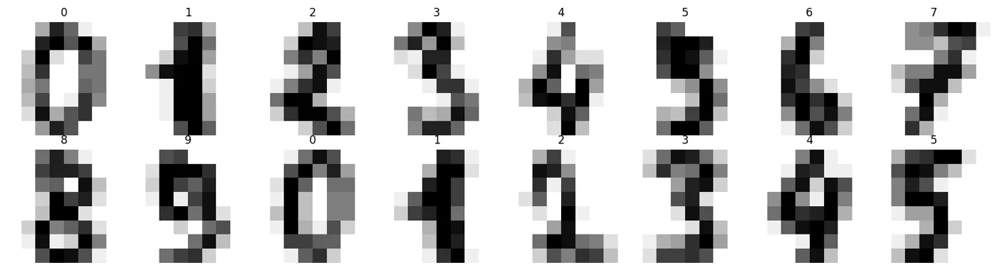
The load_digits dataset: 8x8 pixels, handwritten digits. It ships inside sklearn, no internet needed.
The ordinary network's problem: spatial relationships are lost
nn.Flatten() turns the 8x8 matrix into a 64-element vector. What gets lost?
print("BEFORE Flatten, neighbouring pixels are close to each other:")
print(f"  (3,3) and (3,4) are neighbours -> indices {3*8+3} and {3*8+4} in the vector  (side by side)")
print(f"  (3,3) and (4,3) are neighbours -> indices {3*8+3} and {4*8+3} in the vector  (8 apart!)")
print()
print("To an ordinary Dense layer, 64 elements are just 64 independent numbers.")
print("It does NOT KNOW that 'indices 27 and 35 are vertical neighbours'.")
print()
# proof: we SHUFFLE the pixels and the result doesn't change
r = np.random.default_rng(42)
order = r.permutation(64)
print("Proof: we shuffle the pixels of every image in the SAME order.")
print("If a Dense network doesn't use spatial structure, the result shouldn't change.")
BEFORE Flatten, neighbouring pixels are close to each other:
  (3,3) and (3,4) are neighbours -> indices 27 and 28 in the vector  (side by side)
  (3,3) and (4,3) are neighbours -> indices 27 and 35 in the vector  (8 apart!)

To an ordinary Dense layer, 64 elements are just 64 independent numbers.
It does NOT KNOW that 'indices 27 and 35 are vertical neighbours'.

Proof: we shuffle the pixels of every image in the SAME order.
If a Dense network doesn't use spatial structure, the result shouldn't change.
from sklearn.model_selection import train_test_split
from torch.utils.data import TensorDataset, DataLoader

def build(kind):
    if kind == "dense":
        return nn.Sequential(nn.Flatten(), nn.Linear(64, 128), nn.ReLU(),
                             nn.Dropout(0.2), nn.Linear(128, 10))
    return nn.Sequential(
        nn.Conv2d(1, 16, 3, padding=1), nn.ReLU(), nn.MaxPool2d(2),    # 8x8 -> 4x4
        nn.Conv2d(16, 32, 3, padding=1), nn.ReLU(), nn.MaxPool2d(2),   # 4x4 -> 2x2
        nn.Flatten(), nn.Dropout(0.2), nn.Linear(32 * 2 * 2, 10),
    )

def train(Xtr, ytr, Xte, yte, kind, epochs=30):
    torch.manual_seed(42)
    m = build(kind)
    f = ((lambda a: torch.tensor(a, dtype=torch.float32).unsqueeze(1)) if kind == "cnn"
         else (lambda a: torch.tensor(a, dtype=torch.float32)))
    dl = DataLoader(TensorDataset(f(Xtr), torch.tensor(ytr)), batch_size=64, shuffle=True,
                    generator=torch.Generator().manual_seed(42))
    opt = torch.optim.Adam(m.parameters(), lr=0.003)
    criterion = nn.CrossEntropyLoss()
    for _ in range(epochs):
        m.train()
        for xb, yb in dl:
            opt.zero_grad(); criterion(m(xb), yb).backward(); opt.step()
    m.eval()
    with torch.no_grad():
        acc = float((m(f(Xte)).argmax(1) == torch.tensor(yte)).float().mean())
    return acc, sum(p.numel() for p in m.parameters())

# the version with shuffled pixels
X_shuffled = X_img.reshape(len(X_img), -1)[:, order].reshape(-1, 8, 8)
Xtr, Xte, ytr, yte = train_test_split(X_img, y_img, test_size=.3, random_state=42, stratify=y_img)
Xtr_s, Xte_s, _, _ = train_test_split(X_shuffled, y_img, test_size=.3, random_state=42, stratify=y_img)

a_normal, _ = train(Xtr, ytr, Xte, yte, "dense")
a_shuffled, _ = train(Xtr_s, ytr, Xte_s, yte, "dense")
print(f"Dense, normal images          : {a_normal:.4f}")
print(f"Dense, pixels shuffled        : {a_shuffled:.4f}")
print(f"Difference                    : {a_shuffled - a_normal:+.4f}")
Dense, normal images          : 0.9778
Dense, pixels shuffled        : 0.9741
Difference                    : -0.0037
The result is almost the same, which means the Dense network doesn't use spatial structure at all. Shuffle the image and it doesn't even notice.
A CNN does notice, because it looks at neighbouring pixels.
Convolution: sliding a window
A convolution is a small filter (kernel) that slides over the image and does the same operation everywhere.
def convolve(img_2d, kernel):
    """Convolution by hand, no padding."""
    kh, kw = kernel.shape
    h, w = img_2d.shape
    result = np.zeros((h - kh + 1, w - kw + 1))
    for i in range(result.shape[0]):
        for j in range(result.shape[1]):
            window = img_2d[i:i+kh, j:j+kw]
            result[i, j] = float((window * kernel).sum())     # the operation from Chapter 12!
    return result

# classic filters
kernels = {
    "vertical edge": np.array([[-1, 0, 1], [-1, 0, 1], [-1, 0, 1]], dtype=float),
    "horizontal edge": np.array([[-1, -1, -1], [0, 0, 0], [1, 1, 1]], dtype=float),
    "smoothing": np.ones((3, 3)) / 9,
}
sample = X_img[0]
figure, axes = plt.subplots(1, 4, figsize=(15, 3.6))
axes[0].imshow(sample, cmap="gray_r"); axes[0].set_title(f"original (digit {y_img[0]})"); axes[0].axis("off")
for ax, (name, f_) in zip(axes[1:], kernels.items()):
    ax.imshow(convolve(sample, f_), cmap="gray_r")
    ax.set_title(name, fontsize=10); ax.axis("off")
fig("filtrlar.png", caption="One image, three filters. Each filter sees something different: vertical edges, horizontal edges, smoothness.")

print("Inside a convolution: the dot product from Chapter 12:")
print(f"  result[0,0] = sum(window * kernel)")
print()
print(f"Original image shape   : {sample.shape}")
print(f"After a 3x3 filter     : {convolve(sample, kernels['smoothing']).shape}  (the edges are lost)")
Inside a convolution: the dot product from Chapter 12:
  result[0,0] = sum(window * kernel)

Original image shape   : (8, 8)
After a 3x3 filter     : (6, 6)  (the edges are lost)
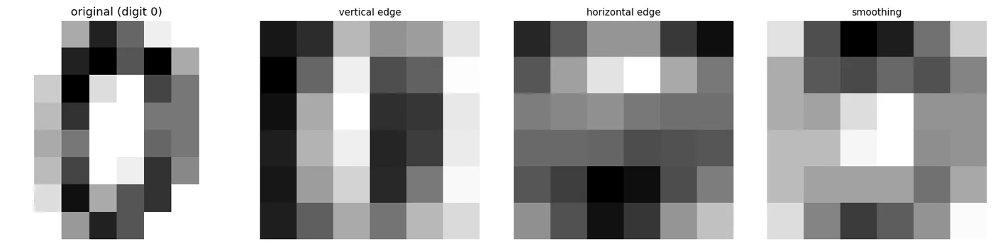
One image, three filters. Each filter sees something different: vertical edges, horizontal edges, smoothness.
A CNN learns the filters ITSELF
I wrote the three filters above by hand: that's the classic computer-vision approach (covered in detail in the OpenCV book).
In a CNN, the filter values are trainable parameters. The model decides for itself: "which filter does this task need?"
So nn.Conv2d(1, 16, 3) is 16 filters of 3x3, all found by gradient descent.
print("Counting the Conv2d parameters:")
conv = nn.Conv2d(1, 16, 3, padding=1)
print(f"  nn.Conv2d(1, 16, 3): {sum(p.numel() for p in conv.parameters())} parameters")
print(f"    = 16 filters x (1 channel x 3 x 3) + 16 biases = {16*9} + 16")
print()
dense_equivalent = 64 * 64
print(f"For comparison: Dense(64, 64) = {dense_equivalent} parameters")
print()
print("That's the CNN's second advantage: WEIGHT SHARING.")
print("One filter is used across the whole image: no separate weight for every position.")
Counting the Conv2d parameters:
  nn.Conv2d(1, 16, 3): 160 parameters
    = 16 filters x (1 channel x 3 x 3) + 16 biases = 144 + 16

For comparison: Dense(64, 64) = 4096 parameters

That's the CNN's second advantage: WEIGHT SHARING.
One filter is used across the whole image: no separate weight for every position.
Pooling: reducing the size
small = X_img[0]
mp = nn.MaxPool2d(2)
ap = nn.AvgPool2d(2)
t = torch.tensor(small, dtype=torch.float32).unsqueeze(0).unsqueeze(0)

figure, axes = plt.subplots(1, 3, figsize=(12, 3.4))
axes[0].imshow(small, cmap="gray_r"); axes[0].set_title(f"original 8x8"); axes[0].axis("off")
axes[1].imshow(mp(t)[0, 0].numpy(), cmap="gray_r"); axes[1].set_title("MaxPool2d(2) -> 4x4"); axes[1].axis("off")
axes[2].imshow(ap(t)[0, 0].numpy(), cmap="gray_r"); axes[2].set_title("AvgPool2d(2) -> 4x4"); axes[2].axis("off")
fig("pooling.png", caption="Pooling halves the size. MaxPool keeps the strongest signal, AvgPool the average.")

print(f"{'step':<28} {'shape'}")
print("-" * 44)
x = t
print(f"{'input':<28} {tuple(x.shape)}")
for name, layer in [("Conv2d(1,16,3,padding=1)", nn.Conv2d(1, 16, 3, padding=1)),
                    ("MaxPool2d(2)", nn.MaxPool2d(2)),
                    ("Conv2d(16,32,3,padding=1)", nn.Conv2d(16, 32, 3, padding=1)),
                    ("MaxPool2d(2)", nn.MaxPool2d(2)),
                    ("Flatten()", nn.Flatten())]:
    x = layer(x)
    print(f"{name:<28} {tuple(x.shape)}")
step                         shape
--------------------------------------------
input                        (1, 1, 8, 8)
Conv2d(1,16,3,padding=1)     (1, 16, 8, 8)
MaxPool2d(2)                 (1, 16, 4, 4)
Conv2d(16,32,3,padding=1)    (1, 32, 4, 4)
MaxPool2d(2)                 (1, 32, 2, 2)
Flatten()                    (1, 128)
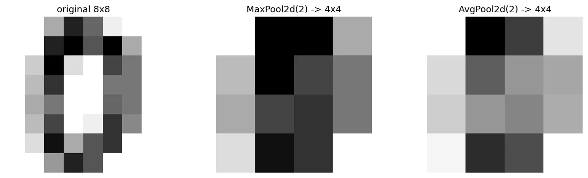
Pooling halves the size. MaxPool keeps the strongest signal, AvgPool the average.
padding and the shape arithmetic: the most common mistake
The output size of Conv2d: (input - kernel + 2*padding) / stride + 1
With padding=1 and a 3x3 kernel the size is kept. Without padding, every convolution loses 2 pixels.
Put three unpadded layers on an 8x8 image: 8 -> 6 -> 4 -> 2. A fourth layer raises an error.
To prevent shape errors, print the shape at every step, like the table above.
The key question: does a CNN really win?
Now we measure. Two cases: the images centred, and shifted.
def shift(images, seed=0):
    """Shift every image randomly by -2..+2 pixels."""
    r_ = np.random.default_rng(seed)
    result = np.zeros_like(images)
    for i, im in enumerate(images):
        dx, dy = r_.integers(-2, 3, 2)
        result[i] = np.roll(np.roll(im, dx, axis=0), dy, axis=1)
    return result

X_shifted = shift(X_img)
figure, axes = plt.subplots(2, 8, figsize=(14, 3.8))
for i in range(8):
    axes[0, i].imshow(X_img[i], cmap="gray_r"); axes[0, i].axis("off")
    axes[1, i].imshow(X_shifted[i], cmap="gray_r"); axes[1, i].axis("off")
axes[0, 0].set_ylabel("original"); axes[1, 0].set_ylabel("shifted")
fig("siljish.png", caption="Top: the centred digits. Bottom: randomly shifted. A person reads both.")
print("In real life an object isn't always in the centre, which is why this test matters.")
In real life an object isn't always in the centre, which is why this test matters.
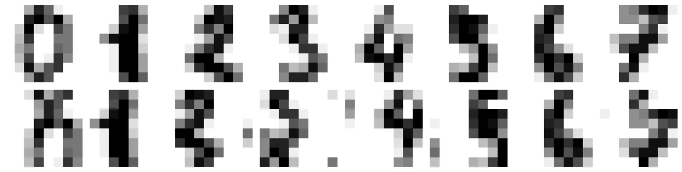
Top: the centred digits. Bottom: randomly shifted. A person reads both.
results = []
for name, Xd in [("centred (original)", X_img), ("SHIFTED", X_shifted)]:
    Xa, Xb, ya, yb = train_test_split(Xd, y_img, test_size=.3, random_state=42, stratify=y_img)
    for kind in ["dense", "cnn"]:
        a, n = train(Xa, ya, Xb, yb, kind)
        results.append({"data": name, "model": kind, "accuracy": round(a, 4), "parameters": n})
show(pd.DataFrame(results))
| data | model | accuracy | parameters |
|---|---|---|---|
| centred (original) | dense | 0.978 | 9 610 |
| centred (original) | cnn | 0.976 | 6 090 |
| SHIFTED | dense | 0.693 | 9 610 |
| SHIFTED | cnn | 0.815 | 6 090 |
Here's the result, and it's more subtle than I expected:
tab = pd.DataFrame(results)
c_dense = tab[(tab["data"].str.startswith("centred")) & (tab.model == "dense")].accuracy.iloc[0]
c_cnn = tab[(tab["data"].str.startswith("centred")) & (tab.model == "cnn")].accuracy.iloc[0]
s_dense = tab[(tab["data"] == "SHIFTED") & (tab.model == "dense")].accuracy.iloc[0]
s_cnn = tab[(tab["data"] == "SHIFTED") & (tab.model == "cnn")].accuracy.iloc[0]
print(f"On centred images: dense {c_dense:.4f}  vs  CNN {c_cnn:.4f}   -> gap {c_cnn-c_dense:+.4f}")
print(f"On shifted images: dense {s_dense:.4f}  vs  CNN {s_cnn:.4f}   -> gap {s_cnn-s_dense:+.4f}")
print()
print(f"CNN parameters  : {tab[tab.model=='cnn'].parameters.iloc[0]}")
print(f"Dense parameters: {tab[tab.model=='dense'].parameters.iloc[0]}")
On centred images: dense 0.9778  vs  CNN 0.9759   -> gap -0.0019
On shifted images: dense 0.6926  vs  CNN 0.8148   -> gap +0.1222

CNN parameters  : 6090
Dense parameters: 9610
On centred images the CNN didn't win: the two are almost equal.
On shifted images the CNN won clearly, and with fewer parameters.
A CNN's advantage isn't "images": it's TRANSLATION INVARIANCE
I started this chapter assuming "a CNN always wins on images". The measurement confirmed that only halfway.
The load_digits images are centred in advance: every digit sits in the middle. Then a Dense network is enough too: it simply memorises rules like "if pixel 27 is bright, this might be a 7".
When the object moves, the rules the Dense network memorised break. A CNN slides the same filter over the whole image, so it finds the object wherever it is.
So you need a CNN when: - the object's position changes (real photographs) - the image is large (at 224x224, a Dense network's parameters explode) - local patterns matter (edges, texture, shape)
And you don't need one for small, centred, uniform images.
Data augmentation: making a CNN stronger
The shifting problem can be solved another way too: by multiplying the training data.
def augment(Xtr_, ytr_, copies=3, seed=1):
    """Make shifted copies of every image."""
    r_ = np.random.default_rng(seed)
    Xs, ys = [Xtr_], [ytr_]
    for k in range(copies):
        Xs.append(shift(Xtr_, seed=seed + k))
        ys.append(ytr_)
    return np.concatenate(Xs), np.concatenate(ys)

Xa, Xb, ya, yb = train_test_split(X_shifted, y_img, test_size=.3, random_state=42, stratify=y_img)
Xa_aug, ya_aug = augment(Xa, ya)
print(f"Train size: {len(Xa)} -> {len(Xa_aug)}  (after augmentation)")
print()
print(f"{'variant':<40} {'accuracy':>9}")
print("-" * 52)
for name, Xt_, yt_, kind in [
    ("dense, NO augmentation", Xa, ya, "dense"),
    ("dense, WITH augmentation", Xa_aug, ya_aug, "dense"),
    ("CNN, NO augmentation", Xa, ya, "cnn"),
    ("CNN, WITH augmentation", Xa_aug, ya_aug, "cnn"),
]:
    a, _ = train(Xt_, yt_, Xb, yb, kind)
    print(f"{name:<40} {a:>9.4f}")
Train size: 1257 -> 5028  (after augmentation)

variant                                   accuracy
----------------------------------------------------
dense, NO augmentation                      0.6926
dense, WITH augmentation                    0.8037
CNN, NO augmentation                        0.8148
CNN, WITH augmentation                      0.9019
Augmentation is the cheapest and most powerful technique when working with images. Without collecting new data, you get more value from the data you have.
Augmentation is applied to TRAIN only
This continues the rule from Chapter 6. You can't augment the test set: you're simulating real conditions, and the test set has to be the real conditions.
In PyTorch this is done with transforms inside the Dataset, so it only touches the train DataLoader.
A typical CNN architecture
show(pd.DataFrame([
    {"Block": "1. Conv + ReLU", "What it does": "Finds local patterns (edges, corners)"},
    {"Block": "2. Conv + ReLU", "What it does": "Builds shapes out of the patterns"},
    {"Block": "3. Pool", "What it does": "Reduces the size, gives tolerance to position"},
    {"Block": "(repeat 1-3)", "What it does": "Each repeat makes the concepts more abstract"},
    {"Block": "4. Flatten", "What it does": "Turns the matrix into a vector"},
    {"Block": "5. Dense + output", "What it does": "The final decision"},
]))
| Block | What it does |
|---|---|
| 1. Conv + ReLU | Finds local patterns (edges, corners) |
| 2. Conv + ReLU | Builds shapes out of the patterns |
| 3. Pool | Reduces the size, gives tolerance to position |
| (repeat 1-3) | Each repeat makes the concepts more abstract |
| 4. Flatten | Turns the matrix into a vector |
| 5. Dense + output | The final decision |
torch.manual_seed(42)
cnn = build("cnn")
print("Our CNN:")
x = torch.zeros(1, 1, 8, 8)
for i, layer in enumerate(cnn):
    x = layer(x)
    name = layer.__class__.__name__
    n_par = sum(p.numel() for p in layer.parameters())
    print(f"  {i}. {name:<12} -> {str(tuple(x.shape)):<18} parameters: {n_par}")
print(f"\nTotal parameters: {sum(p.numel() for p in cnn.parameters())}")
Our CNN:
  0. Conv2d       -> (1, 16, 8, 8)      parameters: 160
  1. ReLU         -> (1, 16, 8, 8)      parameters: 0
  2. MaxPool2d    -> (1, 16, 4, 4)      parameters: 0
  3. Conv2d       -> (1, 32, 4, 4)      parameters: 4640
  4. ReLU         -> (1, 32, 4, 4)      parameters: 0
  5. MaxPool2d    -> (1, 32, 2, 2)      parameters: 0
  6. Flatten      -> (1, 128)           parameters: 0
  7. Dropout      -> (1, 128)           parameters: 0
  8. Linear       -> (1, 10)            parameters: 1290

Total parameters: 6090
Transfer learning: the answer to small data
show(pd.DataFrame([
    {"Situation": "Fewer than 1000 samples", "Solution": "Take a pretrained model, train only the last layer",
     "Name": "Feature extraction"},
    {"Situation": "1000-10000 samples", "Solution": "A pretrained model + train the last blocks too",
     "Name": "Fine-tuning"},
    {"Situation": "100000+ samples", "Solution": "Training from scratch is possible",
     "Name": "Training from scratch"},
]))
print()
print("Why it works: the first layers find edges and textures,")
print("and those are needed just the same in a CAT photo and in an X-RAY.")
print()
print("In practice you take a pretrained model from torchvision.models or HuggingFace.")
print("Because this chapter runs offline, we didn't download one;")
print("you'll see it in full in the YOLO book (stage 11 of the curriculum).")
Why it works: the first layers find edges and textures,
and those are needed just the same in a CAT photo and in an X-RAY.

In practice you take a pretrained model from torchvision.models or HuggingFace.
Because this chapter runs offline, we didn't download one;
you'll see it in full in the YOLO book (stage 11 of the curriculum).
| Situation | Solution | Name |
|---|---|---|
| Fewer than 1000 samples | Take a pretrained model, train only the last layer | Feature extraction |
| 1000-10000 samples | A pretrained model + train the last blocks too | Fine-tuning |
| 100000+ samples | Training from scratch is possible | Training from scratch |
What we learned today
show(pd.DataFrame([
    {"Concept": "Image = matrix", "In one sentence": "8x8 pixels: an ordinary table of numbers"},
    {"Concept": "The problem with Dense", "In one sentence": "Flatten loses the spatial relationships"},
    {"Concept": "Convolution", "In one sentence": "A filter slides over the image: the dot product from Chapter 12"},
    {"Concept": "Weight sharing", "In one sentence": "One filter for the whole image: few parameters"},
    {"Concept": "Pooling", "In one sentence": "Reduces the size, gives tolerance to position"},
    {"Concept": "The CNN's advantage", "In one sentence": "Not images as such: TRANSLATION INVARIANCE"},
    {"Concept": "Centred images", "In one sentence": "Dense is enough too: shown by measurement"},
    {"Concept": "Augmentation", "In one sentence": "The cheapest boost; TRAIN only"},
]))
| Concept | In one sentence |
|---|---|
| Image = matrix | 8x8 pixels: an ordinary table of numbers |
| The problem with Dense | Flatten loses the spatial relationships |
| Convolution | A filter slides over the image: the dot product from Chapter 12 |
| Weight sharing | One filter for the whole image: few parameters |
| Pooling | Reduces the size, gives tolerance to position |
| The CNN's advantage | Not images as such: TRANSLATION INVARIANCE |
| Centred images | Dense is enough too: shown by measurement |
| Augmentation | The cheapest boost; TRAIN only |
The next chapter moves from images to sequences: text, time series, audio.
Questions about this chapter?
The course, homework review and the other five books are in Uzbek. Questions in English are welcome on Telegram.