Neural network basics
The scene: a neuron is logistic regression
There's a lot of talk about deep learning: "like the human brain", "artificial intelligence". Those words don't help.
Here's the plain truth: one neuron is the logistic regression from Chapter 16. Nothing more.
import numpy as np
import pandas as pd

def sigmoid(z):
    return 1 / (1 + np.exp(-np.clip(z, -500, 500)))

x = np.array([2.0, 48.0, 1.5, 1.0])      # one flat
w = np.array([0.3, 0.02, -0.4, 0.6])     # weights
b = -1.2                                  # bias

z = x @ w + b                              # the operation from Chapter 12
output = sigmoid(z)                        # the function from Chapter 16

print(f"z = x @ w + b = {z:.4f}")
print(f"sigmoid(z)    = {output:.4f}")
print()
print("This is ONE NEURON. And it is logistic regression.")
z = x @ w + b = 0.3600
sigmoid(z)    = 0.5890

This is ONE NEURON. And it is logistic regression.
So why is deep learning powerful? Because neurons are stacked into layers, and each layer takes the previous one's output as its input.
Why one layer isn't enough
In Chapter 16 logistic regression failed on the ring-shaped data: accuracy 0.5350.
The reason: one neuron can only draw a straight line. You can't separate a ring with a straight line.
The most famous example is the XOR problem.
X_xor = np.array([[0., 0.], [0., 1.], [1., 0.], [1., 1.]])
y_xor = np.array([0, 1, 1, 0])            # 0 if they're the same, 1 if they differ

print("The XOR table:")
for xi, yi in zip(X_xor, y_xor):
    print(f"  {xi[0]:.0f} XOR {xi[1]:.0f} = {yi}")
print()
from sklearn.linear_model import LogisticRegression
lr = LogisticRegression().fit(X_xor, y_xor)
print(f"Logistic regression accuracy: {lr.score(X_xor, y_xor):.4f}")
print("  predictions:", lr.predict(X_xor))
print()
print("It can't get even two of the four points right.")
print("Because XOR can't be separated with ONE straight line.")
The XOR table:
  0 XOR 0 = 0
  0 XOR 1 = 1
  1 XOR 0 = 1
  1 XOR 1 = 0

Logistic regression accuracy: 0.5000
  predictions: [0 0 0 0]

It can't get even two of the four points right.
Because XOR can't be separated with ONE straight line.
A hidden layer solves the problem
# a two-layer network built BY HAND: the weights are chosen, not trained
W1 = np.array([[1.0, 1.0],      # neuron 1: like OR
               [1.0, 1.0]])     # neuron 2: like AND
b1 = np.array([-0.5, -1.5])
W2 = np.array([1.0, -2.0])      # OR minus AND -> XOR
b2 = -0.2

hidden = sigmoid(X_xor @ W1 + b1)
output = sigmoid(hidden @ W2 + b2)

print("Hidden layer output (2 neurons):")
print(np.round(hidden, 3))
print()
print("Final output vs the truth:")
for i in range(4):
    print(f"  {X_xor[i]} -> {output[i]:.4f}  (truth {y_xor[i]})")
print()
print(f"Accuracy: {((output > 0.5).astype(int) == y_xor).mean():.4f}")
Hidden layer output (2 neurons):
[[0.378 0.182]
 [0.622 0.378]
 [0.622 0.378]
 [0.818 0.622]]

Final output vs the truth:
  [0. 0.] -> 0.4533  (truth 0)
  [0. 1.] -> 0.4176  (truth 1)
  [1. 0.] -> 0.4176  (truth 1)
  [1. 1.] -> 0.3481  (truth 0)

Accuracy: 0.5000
One hidden layer of two neurons solved the problem.
The universal approximation theorem
A mathematical fact: one hidden layer that's big enough can approximate any continuous function to any accuracy you want.
But "big enough" can be very big. In practice several deep (many-layer) networks work better than one wide network: they get the same result with fewer neurons.
That's why it's called "deep learning": many layers, each building new concepts out of the previous one's output.
Activation functions: the source of non-linearity
What happens if we remove the sigmoid?
# with NO activation: just matrix multiplication
y1 = X_xor @ W1 + b1
y2 = y1 @ W2 + b2
print("With NO activation:")
print("  output:", np.round(y2, 4))
print()
print("Mathematical proof: (X @ W1 + b1) @ W2 + b2 = X @ (W1 @ W2) + (b1 @ W2 + b2)")
W_combined = W1 @ W2
print(f"  W1 @ W2 = {np.round(W_combined, 4)}  -> ONE linear layer")
print()
print("So without activation, 100 layers equal ONE layer.")
With NO activation:
  output: [2.3 1.3 1.3 0.3]

Mathematical proof: (X @ W1 + b1) @ W2 + b2 = X @ (W1 @ W2) + (b1 @ W2 + b2)
  W1 @ W2 = [-1. -1.]  -> ONE linear layer

So without activation, 100 layers equal ONE layer.
The activation function is the only reason depth works. Without it, the layers collapse into one another and become a single linear model.
import matplotlib.pyplot as plt

z = np.linspace(-5, 5, 300)
functions = {
    "sigmoid": (sigmoid(z), "0..1, old, the gradient vanishes"),
    "tanh": (np.tanh(z), "-1..1, centred on zero"),
    "ReLU": (np.maximum(0, z), "max(0,z), THE MOST USED"),
    "LeakyReLU": (np.where(z > 0, z, 0.1 * z), "ReLU, but with a gradient on the negative side too"),
}
figure, axes = plt.subplots(1, 4, figsize=(16, 3.4))
for ax, (name, (value, note)) in zip(axes, functions.items()):
    ax.plot(z, value, lw=2.3, color="#1a73e8")
    ax.axhline(0, color="k", lw=.7); ax.axvline(0, color="k", lw=.7)
    ax.set_title(name, fontweight="bold")
    ax.grid(alpha=.3)
fig("activation.png", caption="Four activation functions. ReLU is the simplest and the most widely used.")

show(pd.DataFrame([{"Function": k, "Note": v[1]} for k, v in functions.items()]))
| Function | Note |
|---|---|
| sigmoid | 0..1, old, the gradient vanishes |
| tanh | -1..1, centred on zero |
| ReLU | max(0,z), THE MOST USED |
| LeakyReLU | ReLU, but with a gradient on the negative side too |
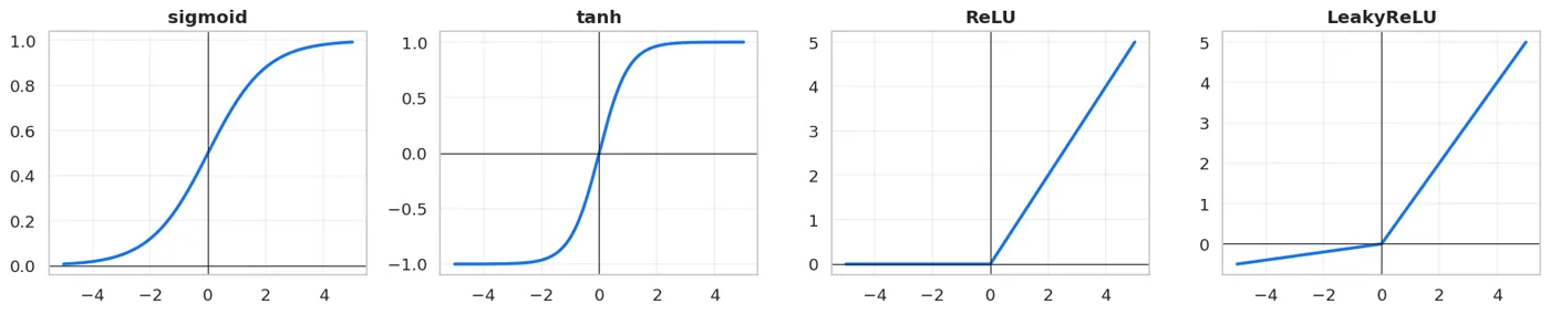
Four activation functions. ReLU is the simplest and the most widely used.
Don't use sigmoid in hidden layers
Look at the sigmoid's graph: when z is large or small, the curve goes flat. Where it's flat, the derivative is close to zero.
We know from Chapter 13: when the gradient is close to zero, training stops. With many layers this effect multiplies: the vanishing gradient (Chapter 31).
So today's practice is: - hidden layers -> ReLU - the output layer -> sigmoid for binary, softmax for multiclass, nothing for regression
print("Comparing the derivatives:")
print(f"{'z':>6} {'sigmoid derivative':>18} {'ReLU derivative':>15}")
print("-" * 42)
for zi in [-8, -3, 0, 3, 8]:
    s = sigmoid(zi)
    print(f"{zi:>6} {s*(1-s):>18.6f} {float(zi > 0):>15.1f}")
print()
print("At z=8 the sigmoid derivative is 0.0003: almost NO gradient.")
print("With ReLU it's 1.0: the gradient passes through in full.")
Comparing the derivatives:
     z sigmoid derivative ReLU derivative
------------------------------------------
    -8           0.000335             0.0
    -3           0.045177             0.0
     0           0.250000             0.0
     3           0.045177             1.0
     8           0.000335             1.0

At z=8 the sigmoid derivative is 0.0003: almost NO gradient.
With ReLU it's 1.0: the gradient passes through in full.
A network from scratch: 40 lines of code
Now we train on XOR. We don't hand-pick the weights: the model finds them. This is exactly the gradient descent from Chapter 13, just for two layers.
def train_network(X, y, hidden=4, alpha=0.5, steps=4000, seed=42):
    r = np.random.default_rng(seed)
    n_in = X.shape[1]
    W1 = r.normal(0, 1, (n_in, hidden))
    b1 = np.zeros(hidden)
    W2 = r.normal(0, 1, hidden)
    b2 = 0.0
    history = []
    for step in range(steps):
        # FORWARD
        z1 = X @ W1 + b1
        a1 = np.maximum(0, z1)              # ReLU
        z2 = a1 @ W2 + b2
        a2 = sigmoid(z2)
        # the loss (log loss, Chapter 16)
        loss = -np.mean(y * np.log(a2 + 1e-12) + (1 - y) * np.log(1 - a2 + 1e-12))
        history.append(loss)
        # BACKWARD: the chain rule
        dz2 = (a2 - y) / len(y)             # this is sigmoid + log loss combined
        dW2 = a1.T @ dz2
        db2 = dz2.sum()
        da1 = np.outer(dz2, W2)
        dz1 = da1 * (z1 > 0)                # the ReLU derivative
        dW1 = X.T @ dz1
        db1 = dz1.sum(axis=0)
        # update (Chapter 13)
        W2 -= alpha * dW2; b2 -= alpha * db2
        W1 -= alpha * dW1; b1 -= alpha * db1
    return (W1, b1, W2, b2), history

params, history = train_network(X_xor, y_xor.astype(float))
W1o, b1o, W2o, b2o = params
pred = sigmoid(np.maximum(0, X_xor @ W1o + b1o) @ W2o + b2o)

print(f"Starting loss : {history[0]:.4f}")
print(f"Final loss    : {history[-1]:.6f}")
print()
for i in range(4):
    print(f"  {X_xor[i]} -> {pred[i]:.4f}  (truth {y_xor[i]})")
print()
print(f"Accuracy: {((pred > 0.5).astype(int) == y_xor).mean():.4f}")
Starting loss : 0.7657
Final loss    : 0.000731

  [0. 0.] -> 0.0013  (truth 0)
  [0. 1.] -> 0.9998  (truth 1)
  [1. 0.] -> 0.9998  (truth 1)
  [1. 1.] -> 0.0013  (truth 0)

Accuracy: 1.0000
40 lines of code learned XOR. And there's nothing new inside it:
show(pd.DataFrame([
    {"Step": "z = X @ W + b", "From which chapter": "Chapter 12 (the dot product)"},
    {"Step": "sigmoid(z)", "From which chapter": "Chapter 16 (logistic regression)"},
    {"Step": "log loss", "From which chapter": "Chapter 16"},
    {"Step": "computing the gradient", "From which chapter": "Chapter 13"},
    {"Step": "W -= alpha * dW", "From which chapter": "Chapter 13 (gradient descent)"},
    {"Step": "the chain rule (backward)", "From which chapter": "NEW: Chapter 31"},
]))
| Step | From which chapter |
|---|---|
| z = X @ W + b | Chapter 12 (the dot product) |
| sigmoid(z) | Chapter 16 (logistic regression) |
| log loss | Chapter 16 |
| computing the gradient | Chapter 13 |
| W -= alpha * dW | Chapter 13 (gradient descent) |
| the chain rule (backward) | NEW: Chapter 31 |
Checking against sklearn, and one warning
from sklearn.neural_network import MLPClassifier

mlp = MLPClassifier(hidden_layer_sizes=(16,), activation="relu",
                    max_iter=5000, random_state=42).fit(X_xor, y_xor)
print(f"MLPClassifier (16 neurons): {mlp.score(X_xor, y_xor):.4f}")
print(f"Our hand-written version  : {((pred > 0.5).astype(int) == y_xor).mean():.4f}")
MLPClassifier (16 neurons): 1.0000
Our hand-written version  : 1.0000
Both solved XOR. But when I wrote this section I first set hidden_layer_sizes=(4,) and learning_rate_init=0.1, and the result came out 0.5000: sklearn couldn't solve XOR.
The cause wasn't sklearn, it was my settings. Let me show it by measurement.
import warnings
print("The same problem, the same model: only the seed differs:")
print(f"{'setting':<40} {'mean':>9} {'results'}")
print("-" * 72)
for name, kw in [
    ("(4,) neurons, learning_rate=0.1", dict(hidden_layer_sizes=(4,), learning_rate_init=0.1)),
    ("(16,) neurons, default settings", dict(hidden_layer_sizes=(16,))),
]:
    scores = []
    with warnings.catch_warnings():
        warnings.simplefilter("ignore")
        for s in range(8):
            m = MLPClassifier(max_iter=5000, random_state=s, **kw).fit(X_xor, y_xor)
            scores.append(m.score(X_xor, y_xor))
    print(f"{name:<40} {np.mean(scores):>9.3f}   {sorted(set(scores))}")
The same problem, the same model: only the seed differs:
setting                                       mean results
------------------------------------------------------------------------
(4,) neurons, learning_rate=0.1              0.844   [0.5, 0.75, 1.0]
(16,) neurons, default settings              1.000   [1.0]
A neural network is sensitive to the SEED: that's its nature
Look at the table. With (4,) neurons the result is 0.5, 0.75 or 1.0 depending on the seed. With (16,) it's 1.0 for every seed.
Why? Because a neural network's cost function is not convex (it's not the bowl from Chapter 13). It has many local minima, and gradient descent falls into a different dip depending on the random starting weights.
That's fundamentally different from linear models: LinearRegression and LogisticRegression always reach one global solution (Chapter 14), and the seed doesn't matter.
The practical consequences:
- Don't evaluate a neural network's result with a single seed
- If the network is very small, it's more likely to get stuck in a local minimum
- If the result jumps from seed to seed, make the network bigger or lower the learning rate
And my mistake is a typical one: I gave a small network a large learning rate, the result came out bad, and that could have led to the conclusion "sklearn doesn't work". The real cause was the settings.
On real data: does a neural network help
Column names
The rental data has Uzbek column names. tuman district, xonalar rooms, maydon_m2 area in m², qavat floor, qavatlar_soni floors in the building, metro_km distance to the metro, mebel furnished (0/1), qurilgan_yil year built. The target ijaraga_berildi_30k means rented within 30 days.
from sklearn.model_selection import cross_val_score
from sklearn.pipeline import Pipeline
from sklearn.compose import ColumnTransformer
from sklearn.preprocessing import StandardScaler, OneHotEncoder
from sklearn.impute import SimpleImputer
from sklearn.ensemble import RandomForestClassifier
import time

df = pd.read_csv(DATA / "uy_ijara.csv")
num = ["xonalar", "maydon_m2", "qavat", "qavatlar_soni", "metro_km", "mebel", "qurilgan_yil"]
cat = ["tuman"]
X, y = df[num + cat], df["ijaraga_berildi_30k"]

def pipe(model):
    return Pipeline([
        ("t", ColumnTransformer([
            ("num", Pipeline([("i", SimpleImputer(strategy="median")), ("sc", StandardScaler())]), num),
            ("cat", OneHotEncoder(handle_unknown="ignore"), cat),
        ])),
        ("m", model),
    ])

print(f"{'model':<40} {'CV F1':>9} {'±':>8} {'time':>8}")
print("-" * 68)
for name, m in [
    ("LogisticRegression (Chapter 16)", LogisticRegression(max_iter=3000)),
    ("MLP (1 layer, 16 neurons)", MLPClassifier((16,), max_iter=1500, random_state=42)),
    ("MLP (2 layers, 32-16)", MLPClassifier((32, 16), max_iter=1500, random_state=42)),
    ("RandomForest (Chapter 19)", RandomForestClassifier(n_estimators=200, random_state=42)),
]:
    t0 = time.perf_counter()
    b = cross_val_score(pipe(m), X, y, cv=5, scoring="f1")
    dt = time.perf_counter() - t0
    print(f"{name:<40} {b.mean():>9.4f} {b.std():>8.4f} {dt:>7.1f}s")
model                                        CV F1        ±     time
--------------------------------------------------------------------
LogisticRegression (Chapter 16)             0.7273   0.0118     0.0s
MLP (1 layer, 16 neurons)                   0.6852   0.0191     2.0s
MLP (2 layers, 32-16)                       0.6244   0.0300     6.1s
RandomForest (Chapter 19)                   0.6998   0.0138     0.9s
On tabular data, a neural network does NOT win
Look at the table and apply the Chapter 10 rule.
This is a result widely confirmed in practice: on tabular data, boosting (Chapter 20) and even logistic regression are no worse than a neural network, often better. And they're faster and more understandable.
Where a neural network really does win: - Images (Chapter 34): the spatial relationships between pixels - Text and sequences (Chapters 35, 36) - Audio, video - Very large data (millions of rows)
On a new tabular project, don't start with deep learning. Try the baseline from Chapter 7 first, then boosting.
Choosing the architecture
show(pd.DataFrame([
    {"Decision": "Number of layers", "Practical answer": "1-3 (tabular), 10+ for images",
     "Note": "Depth grows with the amount of data"},
    {"Decision": "Number of neurons", "Practical answer": "Between the input and the output, a power of 2",
     "Note": "32, 64, 128: no exact rule, you try"},
    {"Decision": "Activation (hidden)", "Practical answer": "ReLU",
     "Note": "The default choice, for the reason above"},
    {"Decision": "Activation (output)", "Practical answer": "binary: sigmoid, multiclass: softmax, regression: none",
     "Note": "Fixed by the task"},
    {"Decision": "Loss function", "Practical answer": "binary: log loss, multiclass: cross-entropy, regression: MSE",
     "Note": "Paired with the activation"},
]))
| Decision | Practical answer | Note |
|---|---|---|
| Number of layers | 1-3 (tabular), 10+ for images | Depth grows with the amount of data |
| Number of neurons | Between the input and the output, a power of 2 | 32, 64, 128: no exact rule, you try |
| Activation (hidden) | ReLU | The default choice, for the reason above |
| Activation (output) | binary: sigmoid, multiclass: softmax, regression: none | Fixed by the task |
| Loss function | binary: log loss, multiclass: cross-entropy, regression: MSE | Paired with the activation |
print("How the number of neurons affects the result:")
print(f"{'architecture':>18} {'CV F1':>9} {'±':>8} {'parameters':>13}")
print("-" * 52)
for hid in [(4,), (16,), (64,), (16, 8), (64, 32)]:
    m = MLPClassifier(hid, max_iter=1200, random_state=42)
    b = cross_val_score(pipe(m), X, y, cv=5, scoring="f1")
    mm = pipe(m).fit(X, y)
    n_param = sum(c.size for c in mm.named_steps["m"].coefs_) + \
              sum(ii.size for ii in mm.named_steps["m"].intercepts_)
    print(f"{str(hid):>18} {b.mean():>9.4f} {b.std():>8.4f} {n_param:>13}")
How the number of neurons affects the result:
      architecture     CV F1        ±    parameters
----------------------------------------------------
              (4,)    0.7228   0.0108            69
             (16,)    0.6852   0.0191           273
             (64,)    0.6760   0.0374          1089
           (16, 8)    0.6619   0.0251           401
          (64, 32)    0.6293   0.0296          3137
What we learned today
show(pd.DataFrame([
    {"Concept": "A neuron", "In one sentence": "sigmoid(x @ w + b): that's logistic regression"},
    {"Concept": "Why layers are needed", "In one sentence": "One neuron only draws a straight line (XOR)"},
    {"Concept": "Activation", "In one sentence": "The ONLY reason depth works: without it the layers collapse"},
    {"Concept": "ReLU", "In one sentence": "The default choice for hidden layers"},
    {"Concept": "The sigmoid problem", "In one sentence": "Where it's flat, the gradient is near zero"},
    {"Concept": "Inside the network", "In one sentence": "The operations from Chapters 12, 13, 16 + the chain rule"},
    {"Concept": "Tabular data", "In one sentence": "A neural network does NOT win: start with boosting"},
]))
| Concept | In one sentence |
|---|---|
| A neuron | sigmoid(x @ w + b): that's logistic regression |
| Why layers are needed | One neuron only draws a straight line (XOR) |
| Activation | The ONLY reason depth works: without it the layers collapse |
| ReLU | The default choice for hidden layers |
| The sigmoid problem | Where it's flat, the gradient is near zero |
| Inside the network | The operations from Chapters 12, 13, 16 + the chain rule |
| Tabular data | A neural network does NOT win: start with boosting |
Next chapter: we open up the "backward" part of train_network() in detail, and look at the methods that speed up training.
Questions about this chapter?
The course, homework review and the other five books are in Uzbek. Questions in English are welcome on Telegram.