RNN, LSTM and time series
The scene: when the order of the rows matters
Until now every row was independent. In the rental data, swap row 5 with row 500 and nothing changes.
Now a different kind of data: a time series. The average rent in Tashkent, month by month.
Here the order is the data. Shuffle it and the information is gone.
import os
os.environ["CUDA_VISIBLE_DEVICES"] = "-1"
import numpy as np
import pandas as pd
import matplotlib.pyplot as plt
import torch
import torch.nn as nn
from torch.utils.data import TensorDataset, DataLoader
from sklearn.linear_model import LinearRegression
from sklearn.neighbors import KNeighborsRegressor
from sklearn.ensemble import RandomForestRegressor
from sklearn.metrics import mean_absolute_error
from sklearn.model_selection import train_test_split

torch.set_num_threads(4)

r = np.random.default_rng(7)
MONTHS = 400
month = np.arange(MONTHS)
series_values = (420 + 0.9 * month + 38 * np.sin(2 * np.pi * month / 12) + r.normal(0, 14, MONTHS)).round(2)
series = pd.Series(series_values, index=pd.date_range("1993-01-01", periods=MONTHS, freq="MS"))

print(f"Series length : {MONTHS} months")
print(f"Range         : {series_values.min():.1f} .. {series_values.max():.1f}")
print(f"First year    : {series_values[:12].mean():.1f}")
print(f"Last year     : {series_values[-12:].mean():.1f}")
print()
print("It contains three things: a TREND (growth), SEASONALITY (a 12-month wave), NOISE.")
Series length : 400 months
Range         : 379.3 .. 827.1
First year    : 423.6
Last year     : 769.7

It contains three things: a TREND (growth), SEASONALITY (a 12-month wave), NOISE.
figure, (a1, a2) = plt.subplots(2, 1, figsize=(12, 6.5))
a1.plot(series.index, series.values, lw=1.1)
a1.set_title("The full series: trend + seasonality")
a1.set_ylabel("price")
a2.plot(series.index[-48:], series.values[-48:], marker="o", ms=3.5, lw=1.2)
a2.set_title("The last 48 months: the seasonality up close")
a2.set_ylabel("price")
plt.tight_layout()
fig("qator.png", caption="A time series: a 12-month seasonal wave on top of a growth trend.")
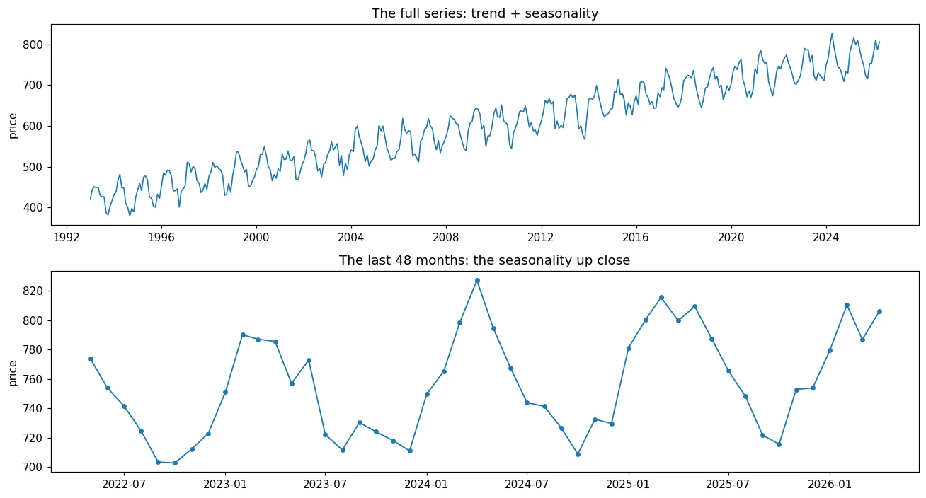
A time series: a 12-month seasonal wave on top of a growth trend.
Lag columns: turning a series into a table
ML models expect a table. The way to turn a time series into a table is a lag window: look at the last L months and predict the next one.
L = 12
X = np.stack([series_values[i:i + L] for i in range(MONTHS - L)])
y = series_values[L:]

print(f"Window length L = {L}")
print(f"X shape: {X.shape}   y shape: {y.shape}")
print()
print("An important observation: neighbouring windows are very similar:")
print(f"  window 0: {X[0][:5]} ...")
print(f"  window 1: {X[1][:5]} ...")
print(f"  values in common: {len(set(X[0]) & set(X[1]))} / {L}")
Window length L = 12
X shape: (388, 12)   y shape: (388,)

An important observation: neighbouring windows are very similar:
  window 0: [420.02 444.08 450.87 448.23 450.14] ...
  window 1: [444.08 450.87 448.23 450.14 429.62] ...
  values in common: 11 / 12
The split: here a random split TELLS LIES
We said in Chapter 6: if the split is wrong, every metric is meaningless. In a time series this mistake comes in another form.
The right way is a chronological split: train first, then test on the following period. Because in practice you predict next month, not last month.
Let's measure it.
cut = int(len(X) * 0.8)
Xtr, Xte, ytr, yte = X[:cut], X[cut:], y[:cut], y[cut:]
Xa, Xb, ya, yb = train_test_split(X, y, test_size=0.2, random_state=42)

print(f"Chronological: train {len(Xtr)} months -> test {len(Xte)} months (the following period)")
print(f"Random       : train {len(Xa)} months -> test {len(Xb)} months (mixed across time)")
print()
print(f"Train target range (chronological): {ytr.min():.1f} .. {ytr.max():.1f}")
print(f"Test  target range (chronological): {yte.min():.1f} .. {yte.max():.1f}")
print()
print(f"{float((yte > ytr.max()).mean()):.1%} of the test set is ABOVE the LARGEST value in train.")
print("So the model has to EXTRAPOLATE: go into a range it has never seen.")
Chronological: train 310 months -> test 78 months (the following period)
Random       : train 310 months -> test 78 months (mixed across time)

Train target range (chronological): 379.3 .. 743.0
Test  target range (chronological): 670.2 .. 827.1

51.3% of the test set is ABOVE the LARGEST value in train.
So the model has to EXTRAPOLATE: go into a range it has never seen.
models = [
    ("linear regression", lambda: LinearRegression()),
    ("KNN (k=3)", lambda: KNeighborsRegressor(3)),
    ("random forest", lambda: RandomForestRegressor(200, random_state=0)),
]
table = []
for name, make in models:
    chrono = mean_absolute_error(yte, make().fit(Xtr, ytr).predict(Xte))
    rand = mean_absolute_error(yb, make().fit(Xa, ya).predict(Xb))
    table.append({"model": name, "chronological MAE": round(chrono, 2),
                  "random MAE": round(rand, 2), "gap": round(rand - chrono, 2)})
show(pd.DataFrame(table))
| model | chronological MAE | random MAE | gap |
|---|---|---|---|
| linear regression | 12.34 | 11.54 | -0.8 |
| KNN (k=3) | 43.9 | 14.22 | -29.68 |
| random forest | 33.33 | 13.95 | -19.38 |
Look at the table. A random split gives every model a "good" result. The chronological split tells the truth: KNN and random forest don't work for this task.
Trees and KNN CANNOT EXTRAPOLATE
I started this section assuming "neighbouring windows are the same, so a random split causes leakage". The measurement rejected that: the cause is something else.
A random forest's prediction is an average of target values from training. KNN's prediction is an average of the nearest neighbours. Neither can go above the largest value seen in training. Mathematically it's impossible.
The series has a trend, so future values are higher than the past. That's why these models get it wrong by their very structure.
Linear regression can extrapolate (it's a line, and a line can be extended), which is why its result is almost the same under both splits.
A random split hides this: the test points get mixed in between the training points, and no extrapolation is needed. You'd see an MAE of 13-14 and ship the model to production. In practice you'd get 33-44.
The rule: in a time series the split is always chronological. And if you want to use tree models on a series with a trend, remove the trend first (differencing).
m_knn = KNeighborsRegressor(3).fit(Xtr, ytr)
m_lin = LinearRegression().fit(Xtr, ytr)
figure, ax = plt.subplots(figsize=(12, 4.2))
ind = np.arange(len(yte))
ax.plot(ind, yte, "k-", lw=2, label="actual")
ax.plot(ind, m_knn.predict(Xte), "--", lw=1.6, label="KNN prediction")
ax.plot(ind, m_lin.predict(Xte), "--", lw=1.6, label="linear regression prediction")
ax.axhline(ytr.max(), color="red", ls=":", lw=1.4, label=f"the maximum in train ({ytr.max():.0f})")
ax.set_title("KNN CANNOT go above the red line")
ax.set_xlabel("test month"); ax.set_ylabel("price"); ax.legend(fontsize=9)
fig("ekstrapolyatsiya.png", caption="The KNN prediction hits the ceiling of the training maximum. Linear regression continues the trend.")
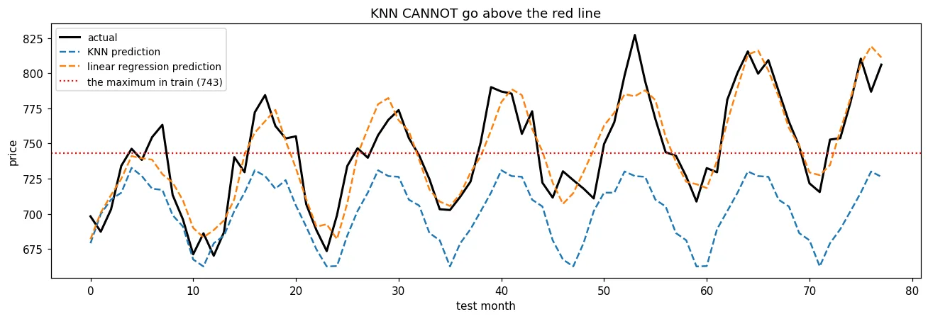
The KNN prediction hits the ceiling of the training maximum. Linear regression continues the trend.
The baseline: the simplest rival for a forecast
The rule from Chapter 7 works here too: baseline first. A time series has two classic baselines.
baselines = {
    "naive (the last value)": Xte[:, -1],
    "seasonal naive (12 months earlier)": Xte[:, 0],
}
result = [{"method": k, "MAE": round(mean_absolute_error(yte, v), 2)} for k, v in baselines.items()]
result.append({"method": "linear regression (12 lags)",
               "MAE": round(mean_absolute_error(yte, m_lin.predict(Xte)), 2)})
show(pd.DataFrame(result))
print("If a complex model doesn't give a lower MAE than THESE numbers, it's unnecessary.")
If a complex model doesn't give a lower MAE than THESE numbers, it's unnecessary.
| method | MAE |
|---|---|
| naive (the last value) | 19.47 |
| seasonal naive (12 months earlier) | 18.25 |
| linear regression (12 lags) | 12.34 |
RNN: a network with memory
Now an architecture built for sequences. An ordinary network sees the whole window at once. An RNN walks through it step by step and keeps a hidden state.
diagramma(
    {
        "x1\nmonth 1": (0.2, 2.5, 1.4, 0.7, "manba"),
        "x2\nmonth 2": (2.1, 2.5, 1.4, 0.7, "manba"),
        "x3\nmonth 3": (4.0, 2.5, 1.4, 0.7, "manba"),
        "h1": (0.2, 1.3, 1.4, 0.7, "qayta"),
        "h2": (2.1, 1.3, 1.4, 0.7, "qayta"),
        "h3": (4.0, 1.3, 1.4, 0.7, "qayta"),
        "answer": (4.0, 0.1, 1.4, 0.7, "xizmat"),
    },
    [("x1\nmonth 1", "h1"), ("x2\nmonth 2", "h2"), ("x3\nmonth 3", "h3"),
     ("h1", "h2", "state"), ("h2", "h3", "state"), ("h3", "answer")],
    nom="rnn_sxema.png",
    izoh="An RNN walks step by step. The hidden state is passed to the right, "
         "and the last state gives the answer. The first month's influence has to travel down this chain.",
)
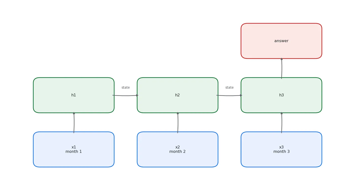
An RNN walks step by step. The hidden state is passed to the right, and the last state gives the answer. The first month's influence has to travel down this chain.
h = 32
rnn = nn.RNN(1, h, batch_first=True)
lstm = nn.LSTM(1, h, batch_first=True)
print(f"nn.RNN(1, {h})  parameters: {sum(p.numel() for p in rnn.parameters())}")
print(f"nn.LSTM(1, {h}) parameters: {sum(p.numel() for p in lstm.parameters())}  (4 times as many: 4 gates)")
print()
print("The LSTM's 4 gates: forget, input, output, and the cell update.")
print("The theory: the gates learn 'what to remember'.")
nn.RNN(1, 32)  parameters: 1120
nn.LSTM(1, 32) parameters: 4480  (4 times as many: 4 gates)

The LSTM's 4 gates: forget, input, output, and the cell update.
The theory: the gates learn 'what to remember'.
A test: long-range memory
The theory says: a plain RNN doesn't remember long sequences, an LSTM does. Let's measure.
The task is deliberately in its purest form: only the first element of the sequence decides the answer. The rest is noise. The model has to hold that one fact all the way to the end of T steps.
def memory_task(n, T, seed=0):
    rr = np.random.default_rng(seed)
    Xs = rr.normal(0, 1, (n, T, 1)).astype(np.float32)
    return torch.tensor(Xs), torch.tensor((Xs[:, 0, 0] > 0).astype(np.int64))

class SeqModel(nn.Module):
    def __init__(self, kind, h=32):
        super().__init__()
        self.rnn = nn.RNN(1, h, batch_first=True) if kind == "rnn" else nn.LSTM(1, h, batch_first=True)
        self.fc = nn.Linear(h, 2)
    def forward(self, x):
        out, _ = self.rnn(x)
        return self.fc(out[:, -1])

def seq_train(kind, T, seed, epochs=60, n=2000):
    torch.manual_seed(seed)
    Xtr_, ytr_ = memory_task(n, T, 1)
    Xte_, yte_ = memory_task(600, T, 2)
    m = SeqModel(kind)
    opt = torch.optim.Adam(m.parameters(), lr=0.005)
    crit = nn.CrossEntropyLoss()
    dl = DataLoader(TensorDataset(Xtr_, ytr_), batch_size=64, shuffle=True,
                    generator=torch.Generator().manual_seed(seed))
    for _ in range(epochs):
        m.train()
        for xb, yb_ in dl:
            opt.zero_grad(); crit(m(xb), yb_).backward(); opt.step()
    m.eval()
    with torch.no_grad():
        return float((m(Xte_).argmax(1) == yte_).float().mean())

print("A random answer = 0.50 accuracy. Each configuration with 3 SEEDS.")
rows = []
for T in [5, 20, 60]:
    for kind in ["rnn", "lstm"]:
        acc = [seq_train(kind, T, s) for s in (0, 1, 2)]
        rows.append({"length T": T, "model": kind,
                     "seeds": str([round(a, 3) for a in acc]),
                     "mean": round(float(np.mean(acc)), 4),
                     "worst": round(min(acc), 4)})
show(pd.DataFrame(rows))
A random answer = 0.50 accuracy. Each configuration with 3 SEEDS.
| length T | model | seeds | mean | worst |
|---|---|---|---|---|
| 5 | rnn | [0.997, 0.995, 0.998] | 0.997 | 0.995 |
| 5 | lstm | [0.998, 0.997, 0.998] | 0.998 | 0.997 |
| 20 | rnn | [0.933, 0.942, 0.838] | 0.904 | 0.838 |
| 20 | lstm | [0.813, 0.493, 0.997] | 0.768 | 0.493 |
| 60 | rnn | [0.847, 0.98, 0.98] | 0.936 | 0.847 |
| 60 | lstm | [0.542, 0.97, 0.517] | 0.676 | 0.517 |
Read the table carefully. I meant to write "LSTM wins on long sequences" in this section. The measurement showed something else.
A conclusion drawn from one seed is no conclusion
The LSTM results are bimodal: on some seeds it solves the task almost completely, on others it stays at the level of random guessing.
That isn't a capacity problem, it's an optimisation problem. The architecture can solve it (the successful seeds prove that), but training doesn't always reach that solution.
There are two practical conclusions:
- Measuring a neural network's result with one seed is the same as not measuring. In Chapter 32 we saw that TensorFlow doesn't reproduce; this is a more serious form of the same problem. Use at least 3 seeds, and record the worst result too.
- "The book says X is good" doesn't mean X is good on your data and within your training budget.
I also tried the classic fix: setting the LSTM's forget-gate bias to 1 (recommended in the literature). In this configuration it didn't help: the result didn't improve. So I didn't put it in the book as a "solution".
Why long range is hard: we measure the gradient
We saw backpropagation in Chapter 31. In a sequence the gradient travels backwards through time, and shrinks along the way.
print("The gradient's size at each input step (T=60, before training):")
print()
for kind in ["rnn", "lstm"]:
    torch.manual_seed(0)
    Xg, yg = memory_task(256, 60, 1)
    Xg.requires_grad_(True)
    m = SeqModel(kind)
    nn.CrossEntropyLoss()(m(Xg), yg).backward()
    g = Xg.grad.abs().mean(dim=(0, 2))
    print(f"  {kind.upper():>5}: step 0 -> {g[0]:.3e} | step 30 -> {g[30]:.3e} | "
          f"step 59 -> {g[59]:.3e}")
    print(f"         the ratio step 59 / step 0: {g[59] / g[0]:.2e}")
The gradient's size at each input step (T=60, before training):

    RNN: step 0 -> 2.427e-17 | step 30 -> 7.964e-11 | step 59 -> 1.129e-05
         the ratio step 59 / step 0: 4.65e+11
   LSTM: step 0 -> 2.503e-17 | step 30 -> 4.343e-11 | step 59 -> 2.982e-05
         the ratio step 59 / step 0: 1.19e+12
There's the root of the problem: the gradient reaching the first step, the one that decides the answer, is many times smaller than at the last step. The model gets far too weak a signal to conclude "the first element matters".
That's why in practice long contexts use neither RNN nor LSTM but attention. It gives every step a direct path. The next chapter is about that.
Is an LSTM useful for forecasting?
Now the main question: on our rent series, does an LSTM beat linear regression?
def lstm_forecast(seed, epochs, difference=False):
    torch.manual_seed(seed)
    if difference:
        Xa, Xb = np.diff(Xtr, axis=1), np.diff(Xte, axis=1)
        ya, base = ytr - Xtr[:, -1], Xte[:, -1]
    else:
        Xa, Xb, ya, base = Xtr, Xte, ytr, 0.0
    mu_, sd_ = Xa.mean(), Xa.std()
    ymu, ysd = ya.mean(), ya.std()
    core = nn.LSTM(1, 32, batch_first=True)
    head = nn.Linear(32, 1)
    opt = torch.optim.Adam(nn.ModuleList([core, head]).parameters(), lr=0.01)
    xt = torch.tensor(((Xa - mu_) / sd_).astype(np.float32)).unsqueeze(-1)
    yt = torch.tensor(((ya - ymu) / ysd).astype(np.float32)).unsqueeze(-1)
    dl = DataLoader(TensorDataset(xt, yt), batch_size=32, shuffle=True,
                    generator=torch.Generator().manual_seed(seed))
    for _ in range(epochs):
        for xb, yb_ in dl:
            opt.zero_grad()
            o, _ = core(xb)
            nn.MSELoss()(head(o[:, -1]), yb_).backward()
            opt.step()
    with torch.no_grad():
        o, _ = core(torch.tensor(((Xb - mu_) / sd_).astype(np.float32)).unsqueeze(-1))
        return head(o[:, -1]).squeeze(-1).numpy() * ysd + ymu + base

experiments = [
    ("LSTM, raw series, 120 epochs", dict(epochs=120)),
    ("LSTM, raw series, 400 epochs", dict(epochs=400)),
    ("LSTM, DIFFERENCED, 400 epochs", dict(epochs=400, difference=True)),
]
final = [
    {"method": "naive (the last value)", "MAE": round(mean_absolute_error(yte, Xte[:, -1]), 2),
     "seeds": "-"},
    {"method": "linear regression (12 lags)",
     "MAE": round(mean_absolute_error(yte, m_lin.predict(Xte)), 2), "seeds": "-"},
]
for name, kw in experiments:
    xs_ = [mean_absolute_error(yte, lstm_forecast(s, **kw)) for s in (0, 1, 2)]
    final.append({"method": name, "MAE": round(float(np.mean(xs_)), 2),
                  "seeds": str([round(v, 1) for v in xs_])})
show(pd.DataFrame(final))
| method | MAE | seeds |
|---|---|---|
| naive (the last value) | 19.47 | - |
| linear regression (12 lags) | 12.34 | - |
| LSTM, raw series, 120 epochs | 30.36 | [40.9, 21.5, 28.7] |
| LSTM, raw series, 400 epochs | 30.73 | [25.9, 33.7, 32.7] |
| LSTM, DIFFERENCED, 400 epochs | 17.87 | [19.8, 15.6, 18.2] |
Three conclusions come out of the table, and the second one stopped me.
First: on the raw series the LSTM does worse than even the naive baseline.
Second: raising the epochs from 120 to 400 didn't help. At first I thought "I gave the LSTM too little training, the comparison is unfair", and tripled the budget. The result didn't change. So the problem isn't the training budget: it's the structure.
Third: after differencing the series, the LSTM improved noticeably.
A neural network can't extrapolate a trend either
Above we saw that KNN and random forest can't go above the training maximum. The LSTM has the same problem, just for a different reason: we normalise the input with the training statistics ((x - mu) / sd). Because the test values lie outside the training range, the model gets inputs of a size it has never seen.
The fix is to make the target the change: not "next month's price" but "how much next month's price differs from the last month". The changes have no trend and stay within a stable range.
In code that's: ya = ytr - Xtr[:, -1], and base = Xte[:, -1] is added back to the prediction.
This is the first thing to do when working with a time series, before choosing a model. In statistics it's called differencing.
For a time series, classic methods first
The same pattern once more in this book: the complex model didn't beat the simple one. Even after differencing, the LSTM stayed below a plain linear regression built on 12 lags.
The practical order for a time series: 1. naive and seasonal naive: the baseline 2. differencing: remove the trend 3. lag columns + linear regression / Ridge: often this is enough 4. ARIMA, Prophet, ETS: statistical methods (outside this book's scope, but they exist) 5. gradient boosting: on the differenced series 6. LSTM / Transformer: when there are many series and lots of data
Choosing an LSTM as your first attempt is the most common mistake.
How to cross-validate correctly
The KFold from Chapter 10 doesn't fit a time series: it puts the future into train and the past into test.
from sklearn.model_selection import TimeSeriesSplit

tss = TimeSeriesSplit(n_splits=5)
print("TimeSeriesSplit: the train window grows, and the test always comes after it:")
print()
print(f"{'fold':>6} {'train':>14} {'test':>14}")
print("-" * 38)
for i, (tr, te) in enumerate(tss.split(X), 1):
    print(f"{i:>6} {f'0..{tr[-1]}':>14} {f'{te[0]}..{te[-1]}':>14}")
print()
xs = [mean_absolute_error(y[te], LinearRegression().fit(X[tr], y[tr]).predict(X[te]))
      for tr, te in tss.split(X)]
print(f"MAE in each fold : {[round(v, 2) for v in xs]}")
print(f"Mean             : {np.mean(xs):.2f}  (+/- {np.std(xs):.2f})")
TimeSeriesSplit: the train window grows, and the test always comes after it:

  fold          train           test
--------------------------------------
     1          0..67        68..131
     2         0..131       132..195
     3         0..195       196..259
     4         0..259       260..323
     5         0..323       324..387

MAE in each fold : [13.75, 11.11, 12.28, 11.82, 12.23]
Mean             : 12.24  (+/- 0.86)
What we learned today
show(pd.DataFrame([
    {"Concept": "The lag window", "In one sentence": "The way to turn a time series into a table"},
    {"Concept": "The chronological split", "In one sentence": "Mandatory: a random split makes the result look good"},
    {"Concept": "Extrapolation", "In one sentence": "Trees and KNN can't go above the training maximum"},
    {"Concept": "Differencing", "In one sentence": "Removing the trend: done BEFORE choosing a model"},
    {"Concept": "TimeSeriesSplit", "In one sentence": "Replaces KFold for a time series"},
    {"Concept": "The time-series baseline", "In one sentence": "naive and seasonal naive: the first rivals"},
    {"Concept": "RNN", "In one sentence": "Walks step by step, keeps a hidden state"},
    {"Concept": "LSTM gates", "In one sentence": "4 times the parameters; long memory in theory"},
    {"Concept": "Seed variance", "In one sentence": "Measured: one seed isn't enough, record the worst"},
    {"Concept": "The vanishing gradient", "In one sentence": "Measured: almost no signal reaches the first step"},
]))
| Concept | In one sentence |
|---|---|
| The lag window | The way to turn a time series into a table |
| The chronological split | Mandatory: a random split makes the result look good |
| Extrapolation | Trees and KNN can't go above the training maximum |
| Differencing | Removing the trend: done BEFORE choosing a model |
| TimeSeriesSplit | Replaces KFold for a time series |
| The time-series baseline | naive and seasonal naive: the first rivals |
| RNN | Walks step by step, keeps a hidden state |
| LSTM gates | 4 times the parameters; long memory in theory |
| Seed variance | Measured: one seed isn't enough, record the worst |
| The vanishing gradient | Measured: almost no signal reaches the first step |
The next chapter shows today's solution to this problem: attention. It doesn't walk along the sequence: it looks at every step at once.
Questions about this chapter?
The course, homework review and the other five books are in Uzbek. Questions in English are welcome on Telegram.