The cost function and gradient descent
The scene: where do the weights come from
In Chapter 12 I wrote the weights by hand:
w = np.array([55.0, 7.5, -28.0, 90.0])
Where did I get them? I made them up. And the prediction came out close, but not exact.
The question: how does the model find these numbers itself?
The answer has two steps:
- Write a function that measures the error (the cost function)
- Search for the weights that make that function as small as possible (gradient descent)
This chapter is the mechanism inside fit().
Column names
The data is synthetic Tashkent rental listings, and its column names are Uzbek. xonalar rooms, maydon_m2 area in m², metro_km distance to the metro, mebel furnished (0/1), narx_usd monthly rent in USD.
Step 1: measure the error
import pandas as pd
import numpy as np
import matplotlib.pyplot as plt

df = pd.read_csv(DATA / "uy_ijara.csv")
num = ["maydon_m2"]                      # ONE feature first, easier to see
X = df[num].to_numpy(dtype=float)
y = df["narx_usd"].to_numpy(dtype=float)

def predict(X, w, b):
    return X @ w + b

def mse(X, y, w, b):
    err = predict(X, w, b) - y
    return float(np.mean(err ** 2))

# a few different guesses
for w_t, b_t in [(np.array([5.0]), 200.0), (np.array([7.5]), 180.0), (np.array([12.0]), 50.0)]:
    print(f"w={w_t[0]:>5.1f}  b={b_t:>5.0f}  ->  MSE = {mse(X, y, w_t, b_t):>12,.0f}".replace(",", " "))
w=  5.0  b=  200  ->  MSE =      105 898
w=  7.5  b=  180  ->  MSE =       41 789
w= 12.0  b=   50  ->  MSE =       14 025
MSE (Mean Squared Error) is the average squared error:
Why squared? Three reasons:
show(pd.DataFrame([
    {"Reason": "Removing the sign", "Note": "A +50 and a -50 error must not cancel each other out"},
    {"Reason": "Punishing big errors more", "Note": "An error of 10 -> 100; an error of 100 -> 10 000"},
    {"Reason": "An easy derivative", "Note": "The derivative of a square is linear, so gradients are convenient"},
]))
| Reason | Note |
|---|---|
| Removing the sign | A +50 and a -50 error must not cancel each other out |
| Punishing big errors more | An error of 10 -> 100; an error of 100 -> 10 000 |
| An easy derivative | The derivative of a square is linear, so gradients are convenient |
MSE is very sensitive to outliers
The square amplifies large errors. If the data has a single price = 999999, it drags the whole MSE, and the whole model, with it.
In that case you use MAE (absolute error) or HuberRegressor. We compare them in Chapter 15.
The cost function is a bowl
Let's draw the MSE for one weight. We fix b and change only w.
w_range = np.linspace(0, 20, 200)
cost = [mse(X, y, np.array([wi]), 180.0) for wi in w_range]
best_i = int(np.argmin(cost))

figure, ax = plt.subplots(figsize=(9.5, 5))
ax.plot(w_range, cost, "b-", lw=2)
ax.plot(w_range[best_i], cost[best_i], "ro", ms=11,
        label=f"lowest: w={w_range[best_i]:.2f}")
ax.set_xlabel("w (the weight of maydon_m2)")
ax.set_ylabel("MSE (cost)")
ax.set_title("The cost function is shaped like a bowl", fontweight="bold")
ax.legend(); ax.grid(alpha=.3)
fig("kosa.png", caption="MSE is shaped like a bowl. The lowest point is the best weight. Gradient descent walks down to it.")

print(f"Lowest point: w = {w_range[best_i]:.3f},  MSE = {cost[best_i]:,.0f}".replace(",", " "))
Lowest point: w = 10.352 MSE = 11 057
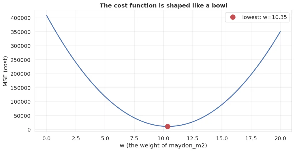
MSE is shaped like a bowl. The lowest point is the best weight. Gradient descent walks down to it.
Now the task is clear: find the bottom of the bowl.
With one weight you can just try 200 values. But with 4 weights that's
So we need another way.
Step 2: the derivative tells you which way is down
Imagine you're on a mountain in thick fog and you want to get down. You can't see the whole valley, but you can feel the slope under your feet.
Whichever way the slope goes down, you step that way. Repeat. You reach the bottom.
The derivative is that slope, in maths.
def gradient(X, y, w, b):
    """The derivatives of MSE with respect to w and b."""
    n = len(y)
    err = predict(X, w, b) - y            # shape (n,)
    dw = (2 / n) * (X.T @ err)            # shape (m,)
    db = (2 / n) * np.sum(err)
    return dw, db

for wi in [3.0, 7.5, 15.0]:
    dw, db = gradient(X, y, np.array([wi]), 180.0)
    direction = "w should GO UP" if dw[0] < 0 else "w should GO DOWN"
    print(f"w={wi:>5.1f}  ->  dw={dw[0]:>12,.1f}   {direction}".replace(",", " "))
w=  3.0  ->  dw=   -54 337.2   w should GO UP
w=  7.5  ->  dw=   -21 257.9   w should GO UP
w= 15.0  ->  dw=    33 874.3   w should GO DOWN
The gradient's sign gives the direction; its size gives the steepness.
The formulas (for a linear model with MSE):
Notice: X.T @ err is the operation from Chapter 12. Nothing new.
Gradient descent: the rule in one line
In words: subtract the gradient from the weight, but first multiply it by a small number. That small number is alpha, the learning rate.
def gradient_descent(X, y, alpha=0.0001, steps=200):
    w = np.zeros(X.shape[1])
    b = 0.0
    history = []
    for i in range(steps):
        dw, db = gradient(X, y, w, b)
        w = w - alpha * dw
        b = b - alpha * db
        history.append({"step": i, "w": float(w[0]), "b": b, "mse": mse(X, y, w, b)})
    return w, b, pd.DataFrame(history)

w_fin, b_fin, history = gradient_descent(X, y, alpha=0.0002, steps=400)
show(history.iloc[[0, 1, 2, 5, 20, 100, 399]].round(3))
| step | w | b | mse |
|---|---|---|---|
| 0 | 19.395 | 0.31 | 156 913.295 |
| 1 | 10.269 | 0.177 | 46 637.126 |
| 2 | 14.563 | 0.253 | 22 220.079 |
| 5 | 13.045 | 0.255 | 15 350.696 |
| 20 | 13.186 | 0.387 | 15 269.7 |
| 100 | 13.176 | 1.078 | 15 239.823 |
| 399 | 13.136 | 3.641 | 15 130.008 |
print(f"Start : w=0.000     MSE={history.mse.iloc[0]:>12,.0f}".replace(",", " "))
print(f"End   : w={w_fin[0]:.3f}   MSE={history.mse.iloc[-1]:>12,.0f}".replace(",", " "))
print()
from sklearn.linear_model import LinearRegression
lr = LinearRegression().fit(X, y)
print(f"sklearn's answer: w={lr.coef_[0]:.3f}  b={lr.intercept_:.2f}")
print(f"Our answer      : w={w_fin[0]:.3f}  b={b_fin:.2f}")
Start : w=0.000     MSE=     156 913
End   : w=13.136   MSE=      15 130

sklearn's answer: w=10.132  b=196.68
Our answer      : w=13.136  b=3.64
Look at the numbers. They don't match:
w: we got 13.136, sklearn 10.132b: we got 3.64, sklearn 196.68
b is terribly far behind: it started at 0, reached only 3.64, and didn't get anywhere near 196.68.
Why? 400 steps aren't enough. But how many is "enough"? Let's measure.
print("How many steps unscaled data needs:")
print(f"{'steps':>10} {'w':>9} {'b':>10} {'MSE':>12}")
print("-" * 44)
for n in [400, 5000, 50000, 300000]:
    w_t, b_t, h_t = gradient_descent(X, y, alpha=0.0002, steps=n)
    mse_text = f"{h_t.mse.iloc[-1]:,.0f}".replace(",", " ")
    print(f"{n:>10} {w_t[0]:>9.3f} {b_t:>10.2f} {mse_text:>12}")
print()
print(f"sklearn:   w={lr.coef_[0]:.3f}  b={lr.intercept_:.2f}")
How many steps unscaled data needs:
     steps         w          b          MSE
--------------------------------------------
       400    13.136       3.64       15 130
      5000    12.584      39.08       13 760
     50000    10.469     175.02       11 072
    300000    10.132     196.68       11 021

sklearn:   w=10.132  b=196.68
It took 300 000 steps. For one feature and 1200 rows.
That price is unacceptable. And the cause is the data's scale: maydon_m2 runs from 22 to 220, so alpha is forced to be tiny, and b's gradient gets multiplied by that same tiny alpha.
The fix comes in the next section.
figure, axes = plt.subplots(1, 2, figsize=(14, 4.8))
axes[0].plot(history.step, history.mse, "b-", lw=2)
axes[0].set_xlabel("Step"); axes[0].set_ylabel("MSE")
axes[0].set_title("The cost falls step by step", fontweight="bold")
axes[0].grid(alpha=.3)

axes[1].plot(w_range, cost, "k-", lw=1.5, alpha=.5, label="cost function")
some_steps = history.iloc[::12]
axes[1].plot(some_steps.w, [mse(X, y, np.array([wi]), 180.0) for wi in some_steps.w],
             "ro-", ms=5, lw=1, label="gradient descent path")
axes[1].set_xlabel("w"); axes[1].set_ylabel("MSE")
axes[1].set_title("Walking down the bowl", fontweight="bold")
axes[1].legend(); axes[1].grid(alpha=.3)
fig("gd_yoli.png", caption="Left: the cost goes down at every step. Right: what those steps look like on the bowl.")
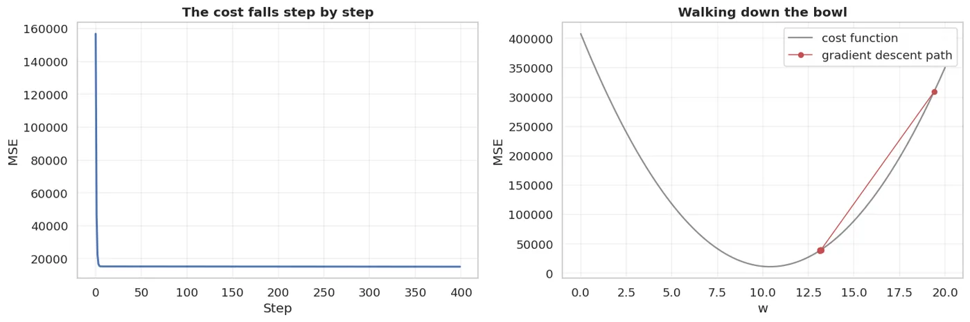
Left: the cost goes down at every step. Right: what those steps look like on the bowl.
The learning rate: the most important setting
If alpha is too small, it's slow. If it's too big, it overshoots the bowl and explodes.
print(f"{'alpha':>10} {'w after 400 steps':>22} {'MSE':>16} {'status':>14}")
print("-" * 68)
for a in [0.000001, 0.00002, 0.0002, 0.001, 0.01]:
    w_t, b_t, h = gradient_descent(X, y, alpha=a, steps=400)
    m = h.mse.iloc[-1]
    if not np.isfinite(m) or m > 1e12:
        status, m_text = "EXPLODED", "inf"
    elif abs(w_t[0] - lr.coef_[0]) < 0.5:
        status, m_text = "converged", f"{m:,.0f}".replace(",", " ")
    else:
        status, m_text = "too slow", f"{m:,.0f}".replace(",", " ")
    print(f"{a:>10} {w_t[0]:>22.3f} {m_text:>16} {status:>14}")
print()
print(f"sklearn's answer: w = {lr.coef_[0]:.3f}")
     alpha      w after 400 steps              MSE         status
--------------------------------------------------------------------
     1e-06                 12.500           17 022       too slow
     2e-05                 13.184           15 263       too slow
    0.0002                 13.136           15 130       too slow
     0.001                    nan              inf       EXPLODED
      0.01                    nan              inf       EXPLODED

sklearn's answer: w = 10.132
The table shows three states: too slow, right, exploded. The window between them is not wide.
Why gradient descent REQUIRES scaling
The alpha values above are tiny: 0.0002. Why?
Because maydon_m2 runs from 22 to 220. The gradient is proportional to that size, so the step has to be very small.
If the columns are on different scales, one alpha can't fit them all: it's too big for one and too small for another. The bowl is "stretched" and gradient descent zigzags.
After StandardScaler, the bowl becomes round and one alpha works for every direction. This is the real reason behind the "scaling is required" rule from Chapter 5.
from sklearn.preprocessing import StandardScaler
Xs = StandardScaler().fit_transform(X)
print("On scaled data a MUCH bigger alpha works:")
print(f"{'alpha':>8} {'w':>10} {'MSE':>14}")
print("-" * 34)
for a in [0.001, 0.01, 0.1, 0.5]:
    w_t, b_t, h = gradient_descent(Xs, y, alpha=a, steps=400)
    print(f"{a:>8} {w_t[0]:>10.2f} {h.mse.iloc[-1]:>13,.0f}".replace(",", " "))
On scaled data a MUCH bigger alpha works:
   alpha          w            MSE
----------------------------------
   0.001     112.41       140 823
    0.01     203.93        11 021
     0.1     203.99        11 021
     0.5     203.99        11 021
After scaling, even alpha=0.1 works. Before scaling, it would have exploded.
With several features
num4 = ["xonalar", "maydon_m2", "metro_km", "mebel"]
X4 = StandardScaler().fit_transform(df[num4].to_numpy(dtype=float))
w4, b4, h4 = gradient_descent(X4, y, alpha=0.1, steps=1500)

lr4 = LinearRegression().fit(X4, y)
compare = pd.DataFrame({
    "feature": num4,
    "we found": w4.round(2),
    "sklearn": lr4.coef_.round(2),
})
show(compare)
print(f"bias: ours {b4:.2f}  |  sklearn {lr4.intercept_:.2f}")
print(f"MSE : ours {h4.mse.iloc[-1]:,.0f}  |  sklearn {mse(X4, y, lr4.coef_, lr4.intercept_):,.0f}".replace(",", " "))
bias: ours 776.10  |  sklearn 776.10
MSE : ours 6 567  |  sklearn 6 567
| feature | we found | sklearn |
|---|---|---|
| xonalar | 62.02 | 62.02 |
| maydon_m2 | 147.32 | 147.32 |
| metro_km | -44.55 | -44.55 |
| mebel | 43.36 | 43.36 |
Nothing in our code changed; X just got more columns. Because gradient() is written with matrix operations, it works with any number of columns.
Three kinds of gradient descent
So far we used all the data at every step. There are other options.
show(pd.DataFrame([
    {"Kind": "Batch GD", "Per step": "ALL rows", "Speed": "Slow",
     "Path": "Smooth", "When": "Small data"},
    {"Kind": "Stochastic GD (SGD)", "Per step": "ONE row", "Speed": "Fast",
     "Path": "Very noisy", "When": "Huge data, online training"},
    {"Kind": "Mini-batch GD", "Per step": "32-256 rows", "Speed": "Fast",
     "Path": "Moderately noisy", "When": "The MOST USED in practice"},
]))
| Kind | Per step | Speed | Path | When |
|---|---|---|---|---|
| Batch GD | ALL rows | Slow | Smooth | Small data |
| Stochastic GD (SGD) | ONE row | Fast | Very noisy | Huge data, online training |
| Mini-batch GD | 32-256 rows | Fast | Moderately noisy | The MOST USED in practice |
def mini_batch_gd(X, y, alpha=0.1, epochs=30, batch=64, seed=42):
    r = np.random.default_rng(seed)
    w, b = np.zeros(X.shape[1]), 0.0
    history = []
    n = len(y)
    for e in range(epochs):
        order = r.permutation(n)
        for start in range(0, n, batch):
            idx = order[start:start + batch]
            dw, db = gradient(X[idx], y[idx], w, b)
            w, b = w - alpha * dw, b - alpha * db
        history.append(mse(X, y, w, b))
    return w, b, history

w_mb, b_mb, hist_mb = mini_batch_gd(X4, y)
print(f"Batch GD      (1500 steps): MSE = {h4.mse.iloc[-1]:>10,.0f}".replace(",", " "))
print(f"Mini-batch GD (30 epochs) : MSE = {hist_mb[-1]:>10,.0f}".replace(",", " "))
print(f"sklearn                   : MSE = {mse(X4, y, lr4.coef_, lr4.intercept_):>10,.0f}".replace(",", " "))
Batch GD      (1500 steps): MSE =      6 567
Mini-batch GD (30 epochs) : MSE =      6 584
sklearn                   : MSE =      6 567
Mini-batch reached a similar result with less computation. Neural networks (Chapters 30–31) use exactly this method.
Why this chapter matters
show(pd.DataFrame([
    {"Where": "Linear regression (Chapter 15)", "Role of gradient descent": "Finds the weights"},
    {"Where": "Logistic regression (Chapter 16)", "Role of gradient descent": "The same, with another cost function"},
    {"Where": "Ridge / Lasso (Chapter 17)", "Role of gradient descent": "A penalty is added to the cost"},
    {"Where": "Neural network (Chapter 31)", "Role of gradient descent": "Backpropagation is the gradient along a chain"},
    {"Where": "XGBoost (Chapter 20)", "Role of gradient descent": "It's in the name: Gradient Boosting"},
]))
| Where | Role of gradient descent |
|---|---|
| Linear regression (Chapter 15) | Finds the weights |
| Logistic regression (Chapter 16) | The same, with another cost function |
| Ridge / Lasso (Chapter 17) | A penalty is added to the cost |
| Neural network (Chapter 31) | Backpropagation is the gradient along a chain |
| XGBoost (Chapter 20) | It's in the name: Gradient Boosting |
You've just learned one mechanism, and it comes back in half the book. Trees (Chapter 18) are the exception; they work in a completely different way.
What we learned today
show(pd.DataFrame([
    {"Concept": "Cost function", "In one sentence": "Measures the error as one number (MSE)"},
    {"Concept": "Why squared", "In one sentence": "Removes the sign, punishes big errors, easy derivative"},
    {"Concept": "The cost is a bowl", "In one sentence": "The task: find the bottom of the bowl"},
    {"Concept": "Gradient", "In one sentence": "The slope: its sign is the direction, its size the steepness"},
    {"Concept": "The GD rule", "In one sentence": "w := w - alpha * gradient"},
    {"Concept": "Learning rate", "In one sentence": "Small is slow, big explodes; the window is narrow"},
    {"Concept": "Why scaling is needed", "In one sentence": "It makes the bowl round, so one alpha works everywhere"},
    {"Concept": "Mini-batch", "In one sentence": "The variant used most in practice"},
]))
| Concept | In one sentence |
|---|---|
| Cost function | Measures the error as one number (MSE) |
| Why squared | Removes the sign, punishes big errors, easy derivative |
| The cost is a bowl | The task: find the bottom of the bowl |
| Gradient | The slope: its sign is the direction, its size the steepness |
| The GD rule | w := w - alpha * gradient |
| Learning rate | Small is slow, big explodes; the window is narrow |
| Why scaling is needed | It makes the bowl round, so one alpha works everywhere |
| Mini-batch | The variant used most in practice |
Next chapter: it turns out linear regression doesn't need gradient descent. You can find the answer with one formula, and we'll see when to choose which.
Questions about this chapter?
The course, homework review and the other five books are in Uzbek. Questions in English are welcome on Telegram.