Logistic regression
The scene: what if we predict 0 and 1 with a linear model
We have two targets. In Chapter 15 we predicted narx_usd with linear regression, successfully.
Now we go back to ijaraga_berildi_30k. It's 0 or 1. The natural question: can we use the same model?
Let's try. It's the quickest lesson there is.
Column names
The data is synthetic Tashkent rental listings, and its column names are Uzbek. xonalar rooms, maydon_m2 area in m², qavat floor, qavatlar_soni floors in the building, metro_km distance to the metro, mebel furnished (0/1). The target ijaraga_berildi_30k means rented within 30 days.
import pandas as pd
import numpy as np
from sklearn.model_selection import train_test_split
from sklearn.linear_model import LinearRegression

df = pd.read_csv(DATA / "uy_ijara.csv")
num = ["xonalar", "maydon_m2", "qavat", "qavatlar_soni", "metro_km", "mebel"]
X, y = df[num], df["ijaraga_berildi_30k"]
X_tr, X_te, y_tr, y_te = train_test_split(X, y, test_size=0.3, random_state=42, stratify=y)

linear = LinearRegression().fit(X_tr, y_tr)
b = linear.predict(X_te)

print(f"The target is only 0 or 1: {sorted(y.unique().tolist())}")
print()
print(f"The linear model's predictions:")
print(f"  smallest : {b.min():.4f}")
print(f"  largest  : {b.max():.4f}")
print()
print(f"Predictions BELOW 0: {int((b < 0).sum())}")
print(f"Predictions ABOVE 1: {int((b > 1).sum())}")
The target is only 0 or 1: [0, 1]

The linear model's predictions:
  smallest : -0.1000
  largest  : 0.9031

Predictions BELOW 0: 7
Predictions ABOVE 1: 0
There's the problem. On our data the model went down to -0.1000: it gave a negative prediction for 7 flats.
"This flat will be rented with a probability of minus 10 percent": that sentence is meaningless.
The upper limit wasn't broken here (the largest prediction is 0.9031). But that's luck: with different data, or with another feature, the model goes above 1 too. Nothing holds a linear function back.
Linear regression doesn't give probabilities
Many students apply LinearRegression to a 0/1 target and read the output as a "probability". That's a mistake: a linear function runs off to infinity, while a probability must stay between 0 and 1.
We need something that forces the output into [0, 1].
The sigmoid: squeezes any number into [0, 1]
import matplotlib.pyplot as plt

def sigmoid(z):
    return 1 / (1 + np.exp(-z))

print(f"{'z':>8} {'sigmoid(z)':>12}   note")
print("-" * 46)
for z in [-6, -2, -1, 0, 1, 2, 6]:
    s = sigmoid(z)
    note = "sticks to 0" if s < 0.05 else ("sticks to 1" if s > 0.95 else
           ("EXACTLY in the middle" if z == 0 else "middle zone"))
    print(f"{z:>8} {s:>12.6f}   {note}")
       z   sigmoid(z)   note
----------------------------------------------
      -6     0.002473   sticks to 0
      -2     0.119203   middle zone
      -1     0.268941   middle zone
       0     0.500000   EXACTLY in the middle
       1     0.731059   middle zone
       2     0.880797   middle zone
       6     0.997527   sticks to 1
z = np.linspace(-8, 8, 300)
figure, axes = plt.subplots(1, 2, figsize=(13.5, 4.6))

axes[0].plot(z, sigmoid(z), "b-", lw=2.5)
axes[0].axhline(0.5, color="gray", ls=":", lw=1)
axes[0].axvline(0, color="gray", ls=":", lw=1)
axes[0].axhline(0, color="red", ls="--", lw=1, alpha=.6)
axes[0].axhline(1, color="red", ls="--", lw=1, alpha=.6)
axes[0].set_xlabel("z = x @ w + b"); axes[0].set_ylabel("sigmoid(z) = probability")
axes[0].set_title("The sigmoid STAYS between 0 and 1", fontweight="bold")
axes[0].grid(alpha=.3)

axes[1].scatter(X_te.maydon_m2, y_te, alpha=.3, s=25, label="truth (0/1)", color="#5f6368")
order = np.argsort(X_te.maydon_m2.to_numpy())
axes[1].plot(X_te.maydon_m2.to_numpy()[order], b[order], "r-", lw=2, label="linear (leaves the bounds)")
from sklearn.pipeline import Pipeline
from sklearn.preprocessing import StandardScaler
from sklearn.linear_model import LogisticRegression
log_one = Pipeline([("sc", StandardScaler()), ("m", LogisticRegression())]).fit(X_tr[["maydon_m2"]], y_tr)
p_one = log_one.predict_proba(X_te[["maydon_m2"]])[:, 1]
axes[1].plot(X_te.maydon_m2.to_numpy()[order], p_one[order], "g-", lw=2.5, label="logistic (inside 0-1)")
axes[1].axhline(0, color="k", ls=":", lw=.8); axes[1].axhline(1, color="k", ls=":", lw=.8)
axes[1].set_xlabel("maydon_m2"); axes[1].set_ylabel("probability")
axes[1].set_title("The two models side by side", fontweight="bold")
axes[1].legend(fontsize=8.5); axes[1].grid(alpha=.3)
fig("sigmoid.png", caption="Left: the sigmoid function. Right: the red line goes below 0 and above 1, while the green line stays within the bounds.")
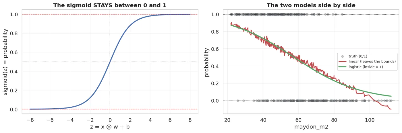
Left: the sigmoid function. Right: the red line goes below 0 and above 1, while the green line stays within the bounds.
Logistic regression = a linear model + the sigmoid:
In other words, x @ w + b from Chapter 12 hasn't changed; one function was added on top.
Why log loss, not MSE
The model gives a probability. How do we measure the error? Can't we use MSE?
def log_loss_one(p, y):
    p = np.clip(p, 1e-15, 1 - 1e-15)
    return -(y * np.log(p) + (1 - y) * np.log(1 - p))

print("When the truth is y=1 and the model gives various probabilities:")
print(f"{'predicted p':>12} {'MSE penalty':>13} {'log loss penalty':>18}")
print("-" * 46)
for p in [0.9, 0.7, 0.5, 0.3, 0.1, 0.01]:
    print(f"{p:>12} {(p - 1)**2:>13.4f} {log_loss_one(p, 1):>18.4f}")
When the truth is y=1 and the model gives various probabilities:
 predicted p   MSE penalty   log loss penalty
----------------------------------------------
         0.9        0.0100             0.1054
         0.7        0.0900             0.3567
         0.5        0.2500             0.6931
         0.3        0.4900             1.2040
         0.1        0.8100             2.3026
        0.01        0.9801             4.6052
There's the difference. The model said p = 0.01, but the truth was 1: it was very confidently, completely wrong.
- The MSE penalty:
0.98, small - The log loss penalty:
4.6, large
Log loss punishes a confident mistake much harder. And that's why the model learns to calibrate its probabilities properly.
The second reason: MSE breaks the bowl
Log loss has another advantage. If you combine the sigmoid with MSE, the cost function is not convex: it grows several dips, and gradient descent can get stuck in a local one (Chapter 13).
The sigmoid with log loss gives a convex bowl, with one global minimum. That's why it was chosen: not only for the penalty, but so that optimisation is reliable.
Coefficients: log-odds and the odds ratio
In linear regression a coefficient was easy to read: "if it goes up by 1 unit, the price changes by this much".
In logistic regression it's different. A coefficient gives the change in log-odds.
pipe = Pipeline([("sc", StandardScaler()), ("m", LogisticRegression(max_iter=2000))]).fit(X_tr, y_tr)
k = pipe.named_steps["m"].coef_[0]

table = pd.DataFrame({
    "feature": num,
    "coefficient (log-odds)": k.round(4),
    "odds ratio (e^k)": np.exp(k).round(4),
}).assign(meaning=lambda d: [
    f"up 1 std -> odds {'up' if v > 1 else 'down'} {abs(v-1)*100:.1f}%"
    for v in d["odds ratio (e^k)"]
])
show(table.sort_values("coefficient (log-odds)", key=abs, ascending=False))
| feature | coefficient (log-odds) | odds ratio (e^k) | meaning |
|---|---|---|---|
| maydon_m2 | -0.945 | 0.389 | up 1 std -> odds down 61.1% |
| xonalar | -0.175 | 0.84 | up 1 std -> odds down 16.0% |
| qavat | 0.086 | 1.09 | up 1 std -> odds up 9.0% |
| metro_km | 0.041 | 1.042 | up 1 std -> odds up 4.2% |
| qavatlar_soni | -0.028 | 0.972 | up 1 std -> odds down 2.8% |
| mebel | -0.021 | 0.979 | up 1 std -> odds down 2.1% |
Odds are p / (1-p). If the probability is 0.75, the odds are 3 ("three to one").
exp(coefficient) is the multiplier on the odds. Above 1, the chances go up; below 1, they go down.
print("How odds and probability are related:")
print(f"{'probability':>12} {'odds':>10} {'log-odds':>11}")
print("-" * 36)
for p in [0.1, 0.25, 0.5, 0.75, 0.9]:
    odds = p / (1 - p)
    print(f"{p:>12} {odds:>10.3f} {np.log(odds):>11.3f}")
print()
print("At p = 0.5 the odds = 1 and the log-odds = 0 -> the centre of the sigmoid")
How odds and probability are related:
 probability       odds    log-odds
------------------------------------
         0.1      0.111      -2.197
        0.25      0.333      -1.099
         0.5      1.000       0.000
        0.75      3.000       1.099
         0.9      9.000       2.197

At p = 0.5 the odds = 1 and the log-odds = 0 -> the centre of the sigmoid
In logistic regression a coefficient does NOT change the probability LINEARLY
"The coefficient is 0.3, so the probability rises by 30%": wrong.
The effect on the probability depends on where you start. Starting from p = 0.5 it moves a lot; starting from p = 0.95 it barely moves, because the sigmoid is flat there.
That's why the odds ratio is used: it's the same multiplier at any point.
Multiclass: when there are three classes
In the Chapter 43 exercise you work with penguins. Logistic regression handles three classes too, in two ways.
from sklearn.impute import SimpleImputer
from sklearn.compose import ColumnTransformer
from sklearn.preprocessing import OneHotEncoder
from sklearn.model_selection import cross_val_score

pg = pd.read_csv(DATA / "penguins.csv")
pnum = ["bill_length_mm", "bill_depth_mm", "flipper_length_mm", "body_mass_g"]
pcat = ["island", "sex"]
Xp, yp = pg[pnum + pcat], pg["species"]

def p_pipe(**kw):
    return Pipeline([
        ("t", ColumnTransformer([
            ("num", Pipeline([("i", SimpleImputer(strategy="median")), ("sc", StandardScaler())]), pnum),
            ("cat", Pipeline([("i", SimpleImputer(strategy="most_frequent")),
                              ("o", OneHotEncoder(handle_unknown="ignore"))]), pcat),
        ])),
        ("m", LogisticRegression(max_iter=3000, **kw)),
    ])

for name, kw in [("multinomial (softmax)", {}), ("one-vs-rest", {"multi_class": "ovr"})]:
    try:
        bb = cross_val_score(p_pipe(**kw), Xp, yp, cv=5, scoring="f1_macro")
        print(f"  {name:24s} macro F1 = {bb.mean():.4f} ±{bb.std():.4f}")
    except Exception as e:
        print(f"  {name:24s} {type(e).__name__}")
  multinomial (softmax)    macro F1 = 0.9939 ±0.0076
  one-vs-rest              macro F1 = 0.9939 ±0.0076
mp = p_pipe().fit(Xp, yp)
print("Classes:", mp.named_steps["m"].classes_.tolist())
print("Coefficient shape:", mp.named_steps["m"].coef_.shape,
      "-> a separate set of coefficients for EACH CLASS")
print()
e = mp.predict_proba(Xp.head(4))
print("Probabilities for the first 4 penguins (each row sums to 1):")
print(pd.DataFrame(e.round(4), columns=mp.named_steps["m"].classes_).to_string(index=False))
print()
print("Row sums:", e.sum(axis=1).round(6).tolist())
Classes: ['Adelie', 'Chinstrap', 'Gentoo']
Coefficient shape: (3, 9) -> a separate set of coefficients for EACH CLASS

Probabilities for the first 4 penguins (each row sums to 1):
 Adelie  Chinstrap  Gentoo
 0.9995     0.0004  0.0001
 0.9911     0.0066  0.0023
 0.9742     0.0234  0.0024
 0.8871     0.0505  0.0625

Row sums: [1.0, 1.0, 1.0, 1.0]
Softmax gives each class a probability, and they add up to exactly 1. Current sklearn versions use it by default.
The threshold: back to Chapter 9
Logistic regression gives a probability. predict() applies the 0.5 threshold. In Chapter 9 we moved that threshold.
from sklearn.metrics import precision_score, recall_score, f1_score, accuracy_score

proba = pipe.predict_proba(X_te)[:, 1]
print(f"{'threshold':>9} {'precision':>11} {'recall':>8} {'F1':>7}")
print("-" * 38)
for t in [0.3, 0.5, 0.7]:
    bb = (proba >= t).astype(int)
    print(f"{t:>9} {precision_score(y_te, bb, zero_division=0):>11.4f} "
          f"{recall_score(y_te, bb, zero_division=0):>8.4f} {f1_score(y_te, bb, zero_division=0):>7.4f}")
print()
print("That's why logistic regression is handy in practice: it gives a probability,")
print("and you choose the threshold to match the business need (Chapter 9).")
threshold   precision   recall      F1
--------------------------------------
      0.3      0.6146   0.9725  0.7532
      0.5      0.7626   0.8297  0.7947
      0.7      0.8554   0.3901  0.5358

That's why logistic regression is handy in practice: it gives a probability,
and you choose the threshold to match the business need (Chapter 9).
When to choose logistic regression
show(pd.DataFrame([
    {"Strength": "Gives a probability", "Why it matters": "You can move the threshold (Chapter 9)"},
    {"Strength": "Explainable", "Why it matters": "The odds ratio: banks and medicine demand it"},
    {"Strength": "Fast and cheap", "Why it matters": "Works even with millions of rows"},
    {"Strength": "Little overfitting", "Why it matters": "A simple model, few parameters"},
    {"Weakness": "ONLY a linear boundary", "Why it matters": "Can't see complex patterns -> a tree (Chapter 18)"},
    {"Weakness": "Needs scaling", "Why it matters": "For the gradient and regularisation"},
    {"Weakness": "Doesn't create features itself", "Why it matters": "Needs manual feature engineering (Chapter 23)"},
]))
| Strength | Why it matters | Weakness |
|---|---|---|
| Gives a probability | You can move the threshold (Chapter 9) | NaN |
| Explainable | The odds ratio: banks and medicine demand it | NaN |
| Fast and cheap | Works even with millions of rows | NaN |
| Little overfitting | A simple model, few parameters | NaN |
| NaN | Can't see complex patterns -> a tree (Chapter 18) | ONLY a linear boundary |
| NaN | For the gradient and regularisation | Needs scaling |
| NaN | Needs manual feature engineering (Chapter 23) | Doesn't create features itself |
Let's see the linear-boundary limitation; it's the bridge to Chapter 18:
from sklearn.tree import DecisionTreeClassifier

# an artificial "ring" pattern: no straight line can separate it
r = np.random.default_rng(42)
n = 600
angle = r.uniform(0, 2 * np.pi, n)
radius = np.where(r.random(n) < 0.5, r.normal(1, .25, n), r.normal(3, .3, n))
Xh = np.c_[radius * np.cos(angle), radius * np.sin(angle)]
yh = (radius > 2).astype(int)

for name, m in [("Logistic Regression", LogisticRegression()),
                ("Decision Tree", DecisionTreeClassifier(max_depth=6, random_state=42))]:
    bb = cross_val_score(Pipeline([("sc", StandardScaler()), ("m", m)]), Xh, yh, cv=5)
    print(f"  {name:22s} accuracy = {bb.mean():.4f} ±{bb.std():.4f}")
print()
print("On ring-shaped data a linear boundary doesn't work.")
print("In Chapter 18 we see how a tree catches a pattern like this.")
  Logistic Regression    accuracy = 0.5350 ±0.0220
  Decision Tree          accuracy = 0.9883 ±0.0085

On ring-shaped data a linear boundary doesn't work.
In Chapter 18 we see how a tree catches a pattern like this.
What we learned today
show(pd.DataFrame([
    {"Concept": "The problem", "In one sentence": "A linear model goes outside 0-1"},
    {"Concept": "Sigmoid", "In one sentence": "Squeezes any number into [0,1]"},
    {"Concept": "The model", "In one sentence": "sigmoid(x @ w + b): the Chapter 12 operation + one function"},
    {"Concept": "Log loss", "In one sentence": "Punishes confident mistakes hard; makes the bowl convex"},
    {"Concept": "Coefficient", "In one sentence": "log-odds; exp(k) = the odds multiplier"},
    {"Concept": "Multiclass", "In one sentence": "Softmax: a probability per class, summing to 1"},
    {"Concept": "Its limitation", "In one sentence": "Only a linear boundary: it can't separate a ring"},
]))
| Concept | In one sentence |
|---|---|
| The problem | A linear model goes outside 0-1 |
| Sigmoid | Squeezes any number into [0,1] |
| The model | sigmoid(x @ w + b): the Chapter 12 operation + one function |
| Log loss | Punishes confident mistakes hard; makes the bowl convex |
| Coefficient | log-odds; exp(k) = the odds multiplier |
| Multiclass | Softmax: a probability per class, summing to 1 |
| Its limitation | Only a linear boundary: it can't separate a ring |
Next chapter: in Chapter 15 the coefficients jumped from split to split. We fix that.
Questions about this chapter?
The course, homework review and the other five books are in Uzbek. Questions in English are welcome on Telegram.