ROC, PR, threshold and imbalanced data
The scene: precision is low, so do we retrain?
In Chapter 8 our model gave precision = 0.7476 and recall = 0.8462. Then the manager walks in:
"The ad budget got cut. When we label a listing 'goes fast', I want that to be right at least 85 percent of the time."
What do you do? Try another algorithm? Collect more data? Order a GPU?
No. You change one number, and you do not retrain the model at all.
That is what this chapter is about. It continues step 10 of the protocol.
Column names
The data is the Tashkent rental listings, and its column names are Uzbek. tuman district, xonalar rooms, maydon_m2 area in m², qavat floor, qavatlar_soni floors in the building, metro_km distance to the metro, mebel furnished (0/1), qurilgan_yil year built. The target ijaraga_berildi_30k means rented within 30 days.
The model does not really output 0 or 1
The first thing to understand: predict() gives you an answer, but the model computes a probability.
import pandas as pd
from sklearn.model_selection import train_test_split
from sklearn.pipeline import Pipeline
from sklearn.compose import ColumnTransformer
from sklearn.preprocessing import StandardScaler, OneHotEncoder
from sklearn.impute import SimpleImputer
from sklearn.linear_model import LogisticRegression

df = pd.read_csv(DATA / "uy_ijara.csv")
num = ["xonalar", "maydon_m2", "qavat", "qavatlar_soni", "metro_km", "mebel", "qurilgan_yil"]
X, y = df[num + ["tuman"]], df["ijaraga_berildi_30k"]
X_tr, X_te, y_tr, y_te = train_test_split(X, y, test_size=0.3, random_state=42, stratify=y)

pipe = Pipeline([
    ("prep", ColumnTransformer([
        ("num", Pipeline([("impute", SimpleImputer(strategy="median")),
                          ("scale", StandardScaler())]), num),
        ("cat", OneHotEncoder(handle_unknown="ignore"), ["tuman"]),
    ])),
    ("model", LogisticRegression(max_iter=2000)),
]).fit(X_tr, y_tr)

proba = pipe.predict_proba(X_te)[:, 1]
compare = pd.DataFrame({"probability": proba.round(3), "predict()": pipe.predict(X_te),
                        "truth": y_te.values}).head(8)
show(compare)
| probability | predict() | truth |
|---|---|---|
| 0.32 | 0 | 1 |
| 0.767 | 1 | 1 |
| 0.65 | 1 | 1 |
| 0.056 | 0 | 0 |
| 0.831 | 1 | 1 |
| 0.615 | 1 | 1 |
| 0.595 | 1 | 0 |
| 0.682 | 1 | 0 |
There is a hidden rule inside predict(): if the probability is above 0.5, answer 1, otherwise 0.
0.5 is not a mathematical truth. It is a default value, and you are allowed to change it.
Moving the threshold
from sklearn.metrics import precision_score, recall_score, f1_score, accuracy_score

print(f"{'threshold':>9} {'precision':>10} {'recall':>8} {'F1':>7} {'accuracy':>9} {'yes count':>10}")
print("-" * 57)
for t in [0.3, 0.4, 0.5, 0.6, 0.7, 0.8]:
    b = (proba >= t).astype(int)
    print(f"{t:>9} {precision_score(y_te, b, zero_division=0):>10.4f} "
          f"{recall_score(y_te, b, zero_division=0):>8.4f} "
          f"{f1_score(y_te, b, zero_division=0):>7.4f} "
          f"{accuracy_score(y_te, b):>9.4f} {int(b.sum()):>10}")
threshold  precision   recall      F1  accuracy  yes count
---------------------------------------------------------
      0.3     0.6181   0.9780  0.7574    0.6833        288
      0.4     0.6748   0.9121  0.7757    0.7333        246
      0.5     0.7476   0.8462  0.7938    0.7778        206
      0.6     0.8027   0.6484  0.7173    0.7417        147
      0.7     0.8370   0.4231  0.5620    0.6667         92
      0.8     0.9189   0.1868  0.3105    0.5806         37
Read the table. As the threshold rises, precision goes up and recall goes down. This is a fixed rule, not a coincidence.
The reason is simple. A higher threshold means the model says "yes" less often. Fewer yeses means it only says yes when it is most confident (precision rises), but it misses many real cases (recall falls).
The manager wants precision ≥ 0.85. Which threshold gets us there?
import numpy as np
needed = None
for t in np.arange(0.30, 0.96, 0.01):
    b = (proba >= t).astype(int)
    if b.sum() > 0 and precision_score(y_te, b, zero_division=0) >= 0.85:
        needed = t
        break
b = (proba >= needed).astype(int)
print(f"Lowest threshold with precision >= 0.85: {needed:.2f}")
print(f"  precision: {precision_score(y_te, b):.4f}")
print(f"  recall   : {recall_score(y_te, b):.4f}")
print(f"  times the model said yes: {int(b.sum())} (it was {int((proba >= 0.5).sum())} at 0.5)")
Lowest threshold with precision >= 0.85: 0.72
  precision: 0.8519
  recall   : 0.3791
  times the model said yes: 81 (it was 206 at 0.5)
There is the answer. We did not retrain the model and we did not change a single line of it. We moved the threshold.
It has a price: recall dropped. What you tell the manager is: "Precision is up to 0.85, but now we will find fewer of the flats that go fast. That is the trade."
Finding the threshold with the best F1 automatically
prec, rec, thr = precision_recall_curve(y_te, proba)
f1 = 2 * prec * rec / np.maximum(prec + rec, 1e-12)
best = int(np.nanargmax(f1[:-1]))
print(thr[best], f1[best])
But careful: a threshold you pick on the test set is optimistic. The right way is to pick it on validation or in CV.
from sklearn.metrics import precision_recall_curve
prec, rec, thr = precision_recall_curve(y_te, proba)
f1_curve = 2 * prec * rec / np.maximum(prec + rec, 1e-12)
best = int(np.nanargmax(f1_curve[:-1]))
print(f"Threshold with the best F1: {thr[best]:.3f}  ->  F1 = {f1_curve[best]:.4f}")
print(f"Default 0.5               :          F1 = {f1_score(y_te, pipe.predict(X_te)):.4f}")
Threshold with the best F1: 0.511  ->  F1 = 0.7979
Default 0.5               :          F1 = 0.7938
Imbalanced data: ROC lies, PR does not
So far the classes were balanced. Now for the case that matters most, because it is the one you meet most often in practice: imbalanced data.
We create the imbalance ourselves: we cut the share of "went fast" down to about 2%.
np.random.seed(42)
fast = y_te[y_te == 1].index
slow = y_te[y_te == 0].index
sample = list(slow) + list(np.random.choice(fast, size=max(1, int(len(slow) * 0.02)), replace=False))

y_imb = y_te.loc[sample]
p_imb = pd.Series(proba, index=y_te.index).loc[sample].values
print(f"New set: {len(y_imb)} rows, share of 'went fast' {y_imb.mean():.2%}")
New set: 181 rows, share of 'went fast' 1.66%
Now we measure two metrics side by side.
from sklearn.metrics import roc_auc_score, average_precision_score

auc = roc_auc_score(y_imb, p_imb)
ap = average_precision_score(y_imb, p_imb)

print(f"ROC-AUC          : {auc:.4f}")
print(f"Average Precision: {ap:.4f}")
print()
print("Baseline for a random model:")
print(f"  ROC-AUC = 0.5000      (ALWAYS, whatever the imbalance)")
print(f"  AP      = {y_imb.mean():.4f}      (= share of the positive class)")
ROC-AUC          : 0.9551
Average Precision: 0.2342

Baseline for a random model:
  ROC-AUC = 0.5000      (ALWAYS, whatever the imbalance)
  AP      = 0.0166      (= share of the positive class)
ROC-AUC looks great. AP is very low.
Why the gap? Look at the formulas.
b_imb = (p_imb >= 0.5).astype(int)
from sklearn.metrics import confusion_matrix
tn, fp, fn, tp = confusion_matrix(y_imb, b_imb).ravel()
print(f"TN={tn}  FP={fp}  FN={fn}  TP={tp}")
print()
print("The second axis of ROC is FPR:")
print(f"  FPR = FP / (FP + TN) = {fp} / ({fp} + {tn}) = {fp/(fp+tn):.4f}")
print()
print("TN is huge (many negatives) -> huge denominator -> FPR is always small.")
print("So the ROC curve hugs the top-left corner and LOOKS BEAUTIFUL.")
print()
print("The PR curve does NOT use TN at all:")
print(f"  precision = TP / (TP + FP) = {tp} / ({tp} + {fp}) = {tp/(tp+fp) if tp+fp else 0:.4f}")
print(f"  recall    = TP / (TP + FN) = {tp} / ({tp} + {fn}) = {tp/(tp+fn) if tp+fn else 0:.4f}")
TN=126  FP=52  FN=0  TP=3

The second axis of ROC is FPR:
  FPR = FP / (FP + TN) = 52 / (52 + 126) = 0.2921

TN is huge (many negatives) -> huge denominator -> FPR is always small.
So the ROC curve hugs the top-left corner and LOOKS BEAUTIFUL.

The PR curve does NOT use TN at all:
  precision = TP / (TP + FP) = 3 / (3 + 52) = 0.0545
  recall    = TP / (TP + FN) = 3 / (3 + 0) = 1.0000
That is the reason. TN is ROC's hidden helper. When negatives are plentiful, it makes ROC look artificially good.
The PR curve only uses TP, FP and FN, so it talks only about the class you care about.
import matplotlib.pyplot as plt
from sklearn.metrics import roc_curve

fpr, tpr, _ = roc_curve(y_imb, p_imb)
p2, r2, _ = precision_recall_curve(y_imb, p_imb)

figure, axes = plt.subplots(1, 2, figsize=(13, 5))
axes[0].plot(fpr, tpr, "b-", lw=2, label=f"AUC = {auc:.3f}")
axes[0].plot([0, 1], [0, 1], "k--", alpha=.5, label="Random (0.5)")
axes[0].set_xlabel("False Positive Rate"); axes[0].set_ylabel("True Positive Rate")
axes[0].set_title("ROC — LOOKS beautiful", color="darkorange", fontweight="bold")
axes[0].legend(); axes[0].grid(alpha=.3)

axes[1].plot(r2, p2, "r-", lw=2, label=f"AP = {ap:.3f}")
axes[1].axhline(y_imb.mean(), color="k", ls="--", alpha=.5, label=f"Random ({y_imb.mean():.3f})")
axes[1].set_xlabel("Recall"); axes[1].set_ylabel("Precision")
axes[1].set_title("PR — shows the TRUTH", color="green", fontweight="bold")
axes[1].legend(); axes[1].grid(alpha=.3)
fig("roc_pr.png", caption="Same model, same data. The chart on the left is lying to you.")
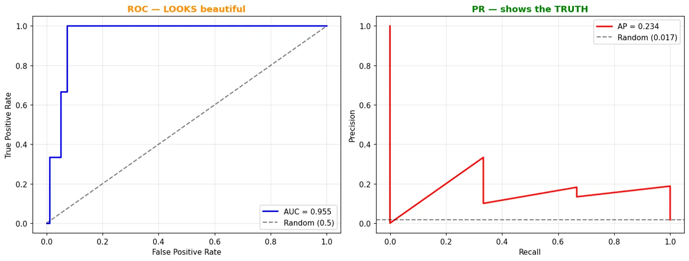
Same model, same data. The chart on the left is lying to you.
When ROC, when PR
- Classes roughly balanced -> ROC-AUC works well and is easy to read.
- Classes imbalanced (positives < 10%) -> use PR-AUC (average precision).
- If a paper reports "AUC 0.92" on imbalanced data, ask for the class ratio.
The rule: if you are looking for something rare (fraud, disease, failure), read PR.
class_weight="balanced" is not a magic fix
The most common advice for "fixing" imbalance is class_weight="balanced". Let's measure it.
idx = list(set(sample))
X_imb = X_te.loc[idx]
y_imb2 = y_te.loc[idx]
X_itr, X_ite, y_itr, y_ite = train_test_split(X_imb, y_imb2, test_size=0.4,
                                              random_state=42, stratify=y_imb2)

def small_pipe(**kw):
    return Pipeline([
        ("prep", ColumnTransformer([
            ("num", Pipeline([("impute", SimpleImputer(strategy="median")),
                              ("scale", StandardScaler())]), num),
            ("cat", OneHotEncoder(handle_unknown="ignore"), ["tuman"]),
        ])),
        ("model", LogisticRegression(max_iter=3000, **kw)),
    ])

plain = small_pipe().fit(X_itr, y_itr)
balanced = small_pipe(class_weight="balanced").fit(X_itr, y_itr)

rows = []
for name, m in [("Plain", plain), ("class_weight=balanced", balanced)]:
    b = m.predict(X_ite)
    rows.append({"Model": name,
                 "Accuracy": round(accuracy_score(y_ite, b), 4),
                 "Precision": round(precision_score(y_ite, b, zero_division=0), 4),
                 "Recall": round(recall_score(y_ite, b, zero_division=0), 4),
                 "F1": round(f1_score(y_ite, b, zero_division=0), 4)})
show(pd.DataFrame(rows))
| Model | Accuracy | Precision | Recall | F1 |
|---|---|---|---|---|
| Plain | 0.986 | 0 | 0 | 0 |
| class_weight=balanced | 0.973 | 0 | 0 | 0 |
What did class_weight="balanced" do? It told the model "mistakes on the rare class cost more". So the model says "yes" more often: recall goes up, precision goes down.
That is not a fix. It is tilting the scales to one side, which is exactly what moving the threshold does too.
There is no such thing as "solving" imbalance
class_weight, SMOTE, oversampling, undersampling: none of them add new knowledge to the data. They only answer the question which mistake do you prefer.
If you have 20 positive examples, no technique turns them into 2000. The fix is to collect more data or to reframe the problem.
macro or weighted: which one do you read
from sklearn.metrics import classification_report
print(classification_report(y_ite, plain.predict(X_ite),
                            target_names=["slow", "fast"], digits=4, zero_division=0))
              precision    recall  f1-score   support

        slow     0.9863    1.0000    0.9931        72
        fast     0.0000    0.0000    0.0000         1

    accuracy                         0.9863        73
   macro avg     0.4932    0.5000    0.4966        73
weighted avg     0.9728    0.9863    0.9795        73
Notice: weighted avg reflects the large class and hides the small one. macro avg counts both classes equally, which is why it is lower and more honest.
The rule: on imbalanced data, read macro.
What we learned today
show(pd.DataFrame([
    {"Concept": "predict() has a 0.5 inside", "In one sentence": "It is a default value, not a mathematical truth"},
    {"Concept": "Moving the threshold", "In one sentence": "Choose precision vs recall without retraining"},
    {"Concept": "Raise the threshold", "In one sentence": "Precision goes up, recall goes down, every time"},
    {"Concept": "ROC-AUC", "In one sentence": "Fine on balanced classes; LIES on imbalanced ones (because of TN)"},
    {"Concept": "PR-AUC (AP)", "In one sentence": "Does not use TN, so it tells the truth on imbalanced data"},
    {"Concept": "class_weight=balanced", "In one sentence": "Not a fix, a tilt of the scales"},
    {"Concept": "macro vs weighted", "In one sentence": "On imbalanced data, read macro"},
]))
| Concept | In one sentence |
|---|---|
| predict() has a 0.5 inside | It is a default value, not a mathematical truth |
| Moving the threshold | Choose precision vs recall without retraining |
| Raise the threshold | Precision goes up, recall goes down, every time |
| ROC-AUC | Fine on balanced classes; LIES on imbalanced ones (because of TN) |
| PR-AUC (AP) | Does not use TN, so it tells the truth on imbalanced data |
| class_weight=balanced | Not a fix, a tilt of the scales |
| macro vs weighted | On imbalanced data, read macro |
Next chapter: every number so far came from one split. Change the split and the numbers change too. That is the problem we solve next.
Questions about this chapter?
The course, homework review and the other five books are in Uzbek. Questions in English are welcome on Telegram.