Attention and the Transformer
The scene: Chapter 35 left us with a problem
In the last chapter we measured it: in a sequence of length T=60, the gradient reaching the first step is billions of times smaller than at the last step. That's why neither the RNN nor the LSTM reliably reached the conclusion "the first element matters".
The root of the problem is the path length. In an RNN, getting from step 1 to step 60 takes 59 multiplications. Every multiplication shrinks the signal.
The idea of the fix is very simple: don't walk. Look at every step directly.
import os
os.environ["CUDA_VISIBLE_DEVICES"] = "-1"
import time
import numpy as np
import pandas as pd
import matplotlib.pyplot as plt
import torch
import torch.nn as nn
from torch.utils.data import TensorDataset, DataLoader

torch.set_num_threads(4)

diagramma(
    {
        "step 1": (0.2, 0.2, 1.3, 0.7, "manba"),
        "...": (1.9, 0.2, 1.3, 0.7, "manba"),
        "step 60": (3.6, 0.2, 1.3, 0.7, "manba"),
        "RNN: walks through\\n59 steps": (0.2, 1.5, 4.7, 0.8, "xizmat"),
        "Attention: a DIRECT\\npath to every step": (0.2, 2.7, 4.7, 0.8, "qayta"),
    },
    [("step 1", "RNN: walks through\\n59 steps"),
     ("step 60", "RNN: walks through\\n59 steps"),
     ("RNN: walks through\\n59 steps", "Attention: a DIRECT\\npath to every step")],
    nom="yol_uzunligi.png",
    izoh="In an RNN information travels along a chain and weakens on the way. "
         "In attention the distance between any two positions is a single step.",
)
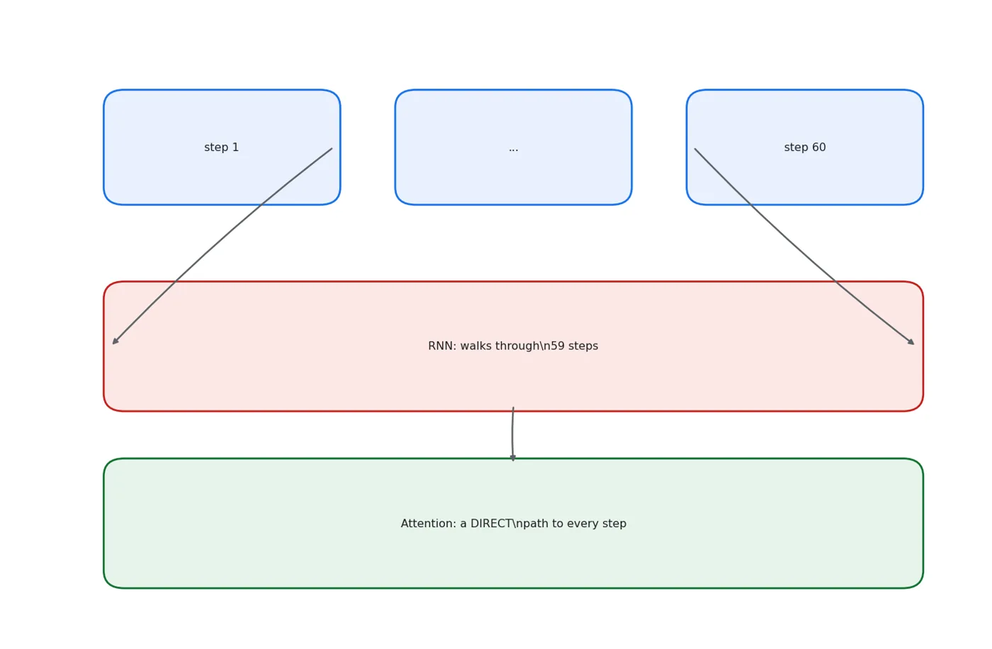
In an RNN information travels along a chain and weakens on the way. In attention the distance between any two positions is a single step.
Attention by hand: three matrices
The whole essence of attention is in one formula. And every operation in that formula was covered in Chapter 12.
Every position builds three vectors:
- Q (query): "what am I looking for?"
- K (key): "what do I have?"
- V (value): "if you take me, this is what you get"
torch.manual_seed(0)
T_small, d = 4, 8
h = torch.randn(1, T_small, d)

Wq, Wk, Wv = (nn.Linear(d, d, bias=False) for _ in range(3))
Q, K, V = Wq(h), Wk(h), Wv(h)
print(f"Input h: {tuple(h.shape)}   -> {T_small} positions, each a {d}-dimensional vector")
print(f"Q, K, V: {tuple(Q.shape)}")
print()

score = Q @ K.transpose(1, 2)
print("Step 1: the dot product of every Q with every K (a similarity score)")
print(f"  score shape: {tuple(score.shape)}  -> every position scores every position")
print(np.round(score[0].detach().numpy(), 2))
print()

score_scaled = score / d ** 0.5
print(f"Step 2: divide by sqrt(d) (d={d}, sqrt={d**0.5:.3f})")
print("  Why: when d is large the scores are large too, and softmax sticks to 0 and 1.")
print()

weight = torch.softmax(score_scaled, dim=-1)
print("Step 3: softmax turns the scores into weights")
print(np.round(weight[0].detach().numpy(), 3))
print(f"  each row sums to: {weight[0].sum(dim=-1).detach().numpy().round(4)}")
print()

output = weight @ V
print(f"Step 4: the weighted average of V -> {tuple(output.shape)}")
print()
print("All in one line:")
print("  softmax(Q @ K.T / sqrt(d)) @ V")
Input h: (1, 4, 8)   -> 4 positions, each a 8-dimensional vector
Q, K, V: (1, 4, 8)

Step 1: the dot product of every Q with every K (a similarity score)
  score shape: (1, 4, 4)  -> every position scores every position
[[ 0.47 -0.97 -0.27 -1.25]
 [-0.46 -0.39 -0.89 -0.09]
 [-0.63 -0.73 -0.3  -0.52]
 [-0.41 -0.08 -0.66 -0.24]]

Step 2: divide by sqrt(d) (d=8, sqrt=2.828)
  Why: when d is large the scores are large too, and softmax sticks to 0 and 1.

Step 3: softmax turns the scores into weights
[[0.343 0.207 0.264 0.187]
 [0.249 0.255 0.213 0.283]
 [0.242 0.234 0.272 0.252]
 [0.244 0.274 0.223 0.259]]
  each row sums to: [1. 1. 1. 1.]

Step 4: the weighted average of V -> (1, 4, 8)

All in one line:
  softmax(Q @ K.T / sqrt(d)) @ V
Attention is a learned average
If you had to put the formula in one sentence: attention is an average whose weights are computed from the data.
In an ordinary average every element gets an equal weight. In attention the weights come from softmax(QK/sqrt(d)), so the model decides every time: "in this situation, which position should I look at?"
That's why it's called "attention".
We measure the gradient flow
In Chapter 35 we measured the gradient for the RNN and the LSTM. Now we put attention through the same measurement.
def task(n, T, seed=0):
    """Only the FIRST element decides the answer. The rest is noise."""
    rr = np.random.default_rng(seed)
    Xs = rr.normal(0, 1, (n, T, 1)).astype(np.float32)
    return torch.tensor(Xs), torch.tensor((Xs[:, 0, 0] > 0).astype(np.int64))

class SeqModel(nn.Module):
    def __init__(self, kind, h=32):
        super().__init__()
        self.rnn = nn.RNN(1, h, batch_first=True) if kind == "rnn" else nn.LSTM(1, h, batch_first=True)
        self.fc = nn.Linear(h, 2)
    def forward(self, x):
        o, _ = self.rnn(x)
        return self.fc(o[:, -1])

class Attention(nn.Module):
    def __init__(self, T, d=32, position=True):
        super().__init__()
        self.inp = nn.Linear(1, d)
        self.pos = nn.Parameter(torch.randn(1, T, d) * 0.02) if position else None
        self.q, self.k, self.v = (nn.Linear(d, d) for _ in range(3))
        self.fc = nn.Linear(d, 2)
        self.weight = None
    def forward(self, x):
        hh = self.inp(x)
        if self.pos is not None:
            hh = hh + self.pos
        Qx, Kx, Vx = self.q(hh), self.k(hh), self.v(hh)
        w = torch.softmax(Qx @ Kx.transpose(1, 2) / Kx.shape[-1] ** 0.5, dim=-1)
        self.weight = w.detach()
        return self.fc((w @ Vx).mean(1))

T = 60
print(f"The gradient reaching the input's first and last steps (T={T}):")
print()
grad_table = []
for name, make in [("RNN", lambda: SeqModel("rnn")), ("LSTM", lambda: SeqModel("lstm")),
                   ("attention", lambda: Attention(T))]:
    torch.manual_seed(0)
    Xg, yg = task(256, T, 1)
    Xg.requires_grad_(True)
    m = make()
    nn.CrossEntropyLoss()(m(Xg), yg).backward()
    g = Xg.grad.abs().mean(dim=(0, 2))
    grad_table.append({"model": name, "step 0": f"{g[0]:.3e}", "step 59": f"{g[59]:.3e}",
                       "step59 / step0": f"{g[59] / g[0]:.2e}"})
show(pd.DataFrame(grad_table))
The gradient reaching the input's first and last steps (T=60):
| model | step 0 | step 59 | step59 / step0 |
|---|---|---|---|
| RNN | 2.427e-17 | 1.129e-05 | 4.65e+11 |
| LSTM | 2.503e-17 | 2.982e-05 | 1.19e+12 |
| attention | 6.268e-06 | 6.604e-06 | 1.05e+00 |
Look at the ratio column. For the RNN and the LSTM it runs into billions, which means the first step gets almost no signal. For attention the ratio is close to one: the gradient reaches every position equally.
The reason is structural: in attention there's one matrix multiplication between step 1 and step 60, not 59.
A test: the same memory task
We repeat the task from Chapter 35, but add attention to the line-up. The conditions are the same: 3 seeds, the same training budget.
def train(make, T_, seed, epochs=60, n=2000, lr=0.005):
    torch.manual_seed(seed)
    Xtr, ytr = task(n, T_, 1)
    Xte, yte = task(600, T_, 2)
    m = make()
    opt = torch.optim.Adam(m.parameters(), lr=lr)
    crit = nn.CrossEntropyLoss()
    dl = DataLoader(TensorDataset(Xtr, ytr), batch_size=64, shuffle=True,
                    generator=torch.Generator().manual_seed(seed))
    for _ in range(epochs):
        m.train()
        for xb, yb in dl:
            opt.zero_grad(); crit(m(xb), yb).backward(); opt.step()
    m.eval()
    with torch.no_grad():
        return float((m(Xte).argmax(1) == yte).float().mean()), m

print("A random answer = 0.50. Every model with 3 seeds.")
test = []
for name, make in [
    ("RNN", lambda: SeqModel("rnn")),
    ("LSTM", lambda: SeqModel("lstm")),
    ("attention (+ position)", lambda: Attention(T)),
    ("attention (NO position)", lambda: Attention(T, position=False)),
]:
    acc = [train(make, T, s)[0] for s in (0, 1, 2)]
    test.append({"model": name, "seeds": str([round(a, 3) for a in acc]),
                 "mean": round(float(np.mean(acc)), 4),
                 "worst": round(min(acc), 4),
                 "parameters": sum(p.numel() for p in make().parameters())})
show(pd.DataFrame(test))
A random answer = 0.50. Every model with 3 seeds.
| model | seeds | mean | worst | parameters |
|---|---|---|---|---|
| RNN | [0.847, 0.98, 0.98] | 0.936 | 0.847 | 1 186 |
| LSTM | [0.542, 0.97, 0.517] | 0.676 | 0.517 | 4 546 |
| attention (+ position) | [0.998, 0.995, 0.998] | 0.997 | 0.995 | 5 218 |
| attention (NO position) | [0.543, 0.56, 0.562] | 0.555 | 0.543 | 3 298 |
The result is clear: attention solves the task on every seed. The LSTM stayed unstable, as we saw in Chapter 35.
But look at the last row of the table: it matters most.
Positional encoding: attention does NOT KNOW the order
The attention (NO position) result is at the level of a random answer. That's not chance.
torch.manual_seed(0)
m_pos = Attention(T, position=False)
Xs, _ = task(8, T, 5)
with torch.no_grad():
    orig = m_pos(Xs)
    shuffled = m_pos(Xs[:, torch.randperm(T)])     # we SHUFFLE the positions

print("Attention without positional encoding: let's shuffle the input:")
print(f"  original output[0] : {orig[0].numpy().round(5)}")
print(f"  shuffled output[0] : {shuffled[0].numpy().round(5)}")
print(f"  maximum difference : {float((orig - shuffled).abs().max()):.2e}")
print()
print("The output didn't change. So to the model a sequence is an UNORDERED SET.")
print("It has no notion of 'the first element', so it can't solve the task.")
Attention without positional encoding: let's shuffle the input:
  original output[0] : [-0.18954  0.12116]
  shuffled output[0] : [-0.18954  0.12116]
  maximum difference : 2.98e-08

The output didn't change. So to the model a sequence is an UNORDERED SET.
It has no notion of 'the first element', so it can't solve the task.
Attention doesn't see order by itself: position has to be added
Look at the formula softmax(QK/sqrt(d)) @ V: the position index takes part nowhere in it. Shuffle the inputs and the outputs just get shuffled too, but their content doesn't change.
The measurement above proved it: on the shuffled input, the output stayed exactly the same.
That's why every transformer adds information about position by hand:
- a learned position vector (what we used:
nn.Parameter) - sine/cosine encoding (in the original "Attention Is All You Need" paper)
- RoPE (widespread in today's LLMs)
Forgetting it is the most common mistake when writing a transformer from scratch. The model trains, the loss goes down, but everything that depends on order breaks.
SHOWING what the model looked at
Attention has one more practical advantage: you can open up the weights and look. In Chapter 26 we explained a model with SHAP; here the explanation is ready-made inside the model.
accuracy, model = train(lambda: Attention(T), T, 0)
Xv, _ = task(200, T, 2)
with torch.no_grad():
    model(Xv)
w = model.weight.mean(dim=(0, 1)).numpy()

print(f"Accuracy of the trained attention model: {accuracy:.4f}")
print()
print(f"Average attention on step 0           : {w[0]:.4f}")
print(f"Average over the other 59 steps       : {w[1:].mean():.6f}")
print(f"The step that got the most attention  : {int(w.argmax())}")
print()
print("The model found it by itself: the answer is at the FIRST step. We gave it no hint.")
Accuracy of the trained attention model: 0.9983

Average attention on step 0           : 0.9975
Average over the other 59 steps       : 0.000042
The step that got the most attention  : 0

The model found it by itself: the answer is at the FIRST step. We gave it no hint.
figure, (b1, b2) = plt.subplots(1, 2, figsize=(14, 4.2),
                                gridspec_kw={"width_ratios": [1.15, 1]})
b1.bar(np.arange(T), w, color="#1a73e8")
b1.set_title("Average attention given to each step")
b1.set_xlabel("sequence step"); b1.set_ylabel("weight")
image = b2.imshow(model.weight[0].numpy(), cmap="viridis", aspect="auto")
b2.set_title("The attention matrix (one sample)")
b2.set_xlabel("step being looked at"); b2.set_ylabel("query step")
plt.colorbar(image, ax=b2, fraction=0.046)
plt.tight_layout()
fig("attention_ogirligi.png",
    caption="Left: all the attention is concentrated on step 0. Right: the attention matrix's "
            "left column is bright: every position looks at step 0.")
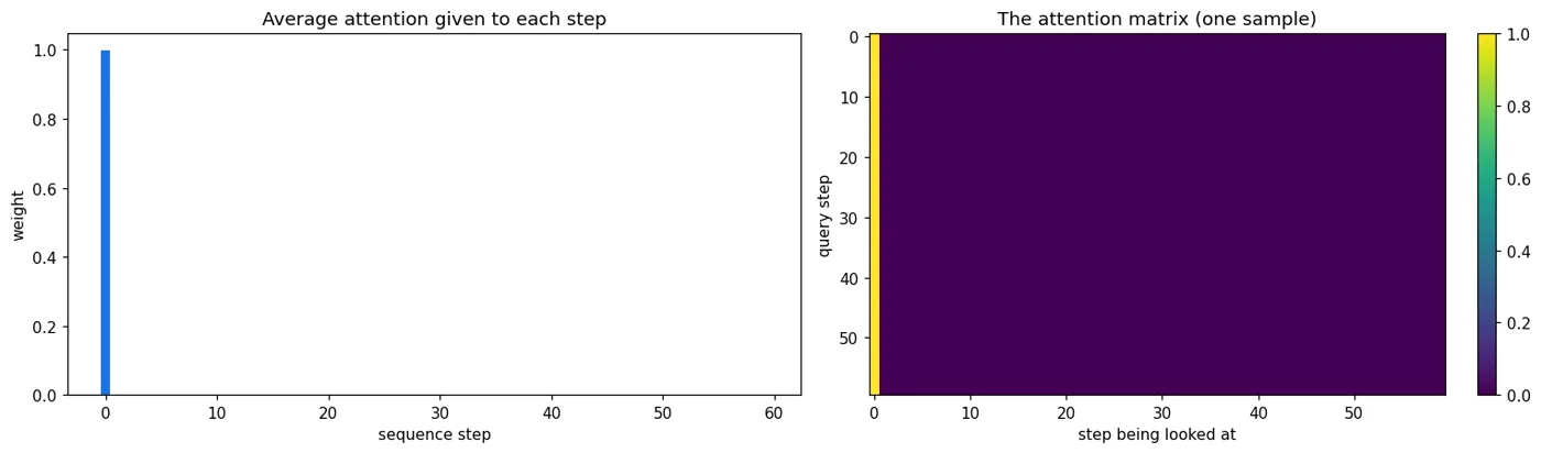
Left: all the attention is concentrated on step 0. Right: the attention matrix's left column is bright: every position looks at step 0.
The cost: O(T squared)
Attention isn't free. It compares every position with every position, which means it builds a T x T matrix. Let's measure that.
print(f"{'T':>6} {'RNN time (ms)':>16} {'attention (ms)':>16} {'attn matrix size':>22}")
print("-" * 64)
for Tx in [30, 60, 120, 240]:
    Xb, _ = task(64, Tx, 3)
    r_m, a_m = SeqModel("rnn"), Attention(Tx)
    with torch.no_grad():
        r_m(Xb); a_m(Xb)                                   # warm-up
        t0 = time.perf_counter(); [r_m(Xb) for _ in range(10)]
        t_rnn = (time.perf_counter() - t0) * 100
        t0 = time.perf_counter(); [a_m(Xb) for _ in range(10)]
        t_attn = (time.perf_counter() - t0) * 100
    print(f"{Tx:>6} {t_rnn:>16.2f} {t_attn:>16.2f} {f'{Tx}x{Tx} = {Tx*Tx}':>22}")
print()
print("The matrix size column: when T doubles, it grows EXACTLY fourfold.")
print("The time columns say something else: read the note below.")
     T    RNN time (ms)   attention (ms)       attn matrix size
----------------------------------------------------------------
    30             0.32             0.17            30x30 = 900
    60             0.58             0.30           60x60 = 3600
   120             1.08             0.68        120x120 = 14400
   240             2.09             3.88        240x240 = 57600

The matrix size column: when T doubles, it grows EXACTLY fourfold.
The time columns say something else: read the note below.
The measurement half-rejected my assumption
I put this table here for the conclusion "attention is expensive". The result came out differently: at small T, attention runs faster than the RNN.
The reason is parallelism. An RNN has to go through its T steps one after another: 240 steps means 240 operations waiting in a queue. Attention does all of it in one big matrix multiplication, and matrix multiplication is extremely well optimised.
The quadratic growth only takes over when T is large. In the table the crossover point appears between 120 and 240.
So the right conclusion has two parts:
- On speed attention wins: that's why transformers replaced RNNs. You can train them in parallel on a GPU; you can't do that with an RNN.
- On memory and long contexts the quadratic growth is a real barrier: you have to store the T x T matrix. For a 100 000-token context that's 10 billion elements.
That second reason is why methods like FlashAttention, sliding-window attention and MQA appeared: they solve exactly the memory problem, not speed.
The general lesson: the word "expensive" means nothing without a measurement. Expensive in what: time, memory, or parameters?
The Transformer block
Attention is one brick. A Transformer block adds four things around it.
show(pd.DataFrame([
    {"Part": "1. Multi-head attention",
     "Job": "Several attentions in parallel: each looks at a different relationship"},
    {"Part": "2. A residual connection (x + attn(x))",
     "Job": "Gives the gradient a direct path: required for a deep network"},
    {"Part": "3. LayerNorm",
     "Job": "Stabilises each layer's output"},
    {"Part": "4. Feed-forward (a 2-layer MLP)",
     "Job": "Processes the information attention gathered"},
]))
print()
print("This block is stacked N times. GPT, BERT, Llama: all variants of this pattern.")
print("The differences: the number of blocks, the size, the kind of positional encoding, and the attention mask.")
This block is stacked N times. GPT, BERT, Llama: all variants of this pattern.
The differences: the number of blocks, the size, the kind of positional encoding, and the attention mask.
| Part | Job |
|---|---|
| 1. Multi-head attention | Several attentions in parallel: each looks at a different relationship |
| 2. A residual connection (x + attn(x)) | Gives the gradient a direct path: required for a deep network |
| 3. LayerNorm | Stabilises each layer's output |
| 4. Feed-forward (a 2-layer MLP) | Processes the information attention gathered |
class TransformerBlock(nn.Module):
    """Minimal but complete: attention + residual + norm + feed-forward."""
    def __init__(self, d=32, heads=4):
        super().__init__()
        self.attn = nn.MultiheadAttention(d, heads, batch_first=True)
        self.norm1, self.norm2 = nn.LayerNorm(d), nn.LayerNorm(d)
        self.ff = nn.Sequential(nn.Linear(d, 4 * d), nn.GELU(), nn.Linear(4 * d, d))
    def forward(self, x):
        a, _ = self.attn(x, x, x)
        x = self.norm1(x + a)                 # residual + norm
        return self.norm2(x + self.ff(x))     # residual + norm

block = TransformerBlock()
sample = torch.randn(2, 10, 32)
print(f"Input : {tuple(sample.shape)}")
print(f"Output: {tuple(block(sample).shape)}   (the shape is kept, which is why blocks can be stacked)")
print(f"Parameters: {sum(p.numel() for p in block.parameters())}")
print()
print("nn.MultiheadAttention is a ready-made, faster version of the formula we wrote by hand.")
Input : (2, 10, 32)
Output: (2, 10, 32)   (the shape is kept, which is why blocks can be stacked)
Parameters: 12704

nn.MultiheadAttention is a ready-made, faster version of the formula we wrote by hand.
What you can do with it
show(pd.DataFrame([
    {"Task": "Text classification", "Approach": "A pretrained model + the last layer (fine-tuning)"},
    {"Task": "Question-answering over your own documents", "Approach": "RAG: retrieval + an LLM"},
    {"Task": "Text in your own style", "Approach": "LoRA fine-tuning"},
    {"Task": "Text from images (OCR)", "Approach": "A vision transformer + a decoder"},
    {"Task": "A time series", "Approach": "Chapter 35 first: differencing and classic methods"},
]))
print()
print("Important: in none of these tasks do you train a transformer FROM SCRATCH.")
print("You take a pretrained model and adapt it. How to do that is in Chapter 39 (LoRA, QLoRA).")
Important: in none of these tasks do you train a transformer FROM SCRATCH.
You take a pretrained model and adapt it. How to do that is in Chapter 39 (LoRA, QLoRA).
| Task | Approach |
|---|---|
| Text classification | A pretrained model + the last layer (fine-tuning) |
| Question-answering over your own documents | RAG: retrieval + an LLM |
| Text in your own style | LoRA fine-tuning |
| Text from images (OCR) | A vision transformer + a decoder |
| A time series | Chapter 35 first: differencing and classic methods |
Training from scratch isn't your job
In the measurements above, our attention model solved an artificial task of length 60. A real language model needs billions of tokens and thousands of GPU-hours.
The practical work is adapting a pretrained model. That's why the next part of this book (Chapters 37-41) builds exactly that chain: collecting data, building a dataset, fine-tuning, saving, and serving.
And you need the theory for this: why there's a context limit, why a long prompt is expensive, why position matters, why a model sometimes "forgets" an instruction at the start. The answers to those questions are in this chapter's formula.
What we learned today
show(pd.DataFrame([
    {"Concept": "The attention formula", "In one sentence": "softmax(Q @ K.T / sqrt(d)) @ V"},
    {"Concept": "Q, K, V", "In one sentence": "Query, key, value: all three are linear projections"},
    {"Concept": "Why sqrt(d)", "In one sentence": "Keeps the softmax from saturating"},
    {"Concept": "Path length", "In one sentence": "One step between any positions, not 59"},
    {"Concept": "Gradient flow", "In one sentence": "Measured: the ratio is close to one, billions for the RNN"},
    {"Concept": "Positional encoding", "In one sentence": "Measured: without it the model can't see order"},
    {"Concept": "Explanation", "In one sentence": "The weights show where the model looked"},
    {"Concept": "O(T squared)", "In one sentence": "The matrix grows 4x: the barrier is MEMORY, not speed"},
    {"Concept": "Parallelism", "In one sentence": "Measured: at small T attention is faster than an RNN"},
    {"Concept": "The Transformer block", "In one sentence": "Attention + residual + norm + feed-forward"},
]))
| Concept | In one sentence |
|---|---|
| The attention formula | softmax(Q @ K.T / sqrt(d)) @ V |
| Q, K, V | Query, key, value: all three are linear projections |
| Why sqrt(d) | Keeps the softmax from saturating |
| Path length | One step between any positions, not 59 |
| Gradient flow | Measured: the ratio is close to one, billions for the RNN |
| Positional encoding | Measured: without it the model can't see order |
| Explanation | The weights show where the model looked |
| O(T squared) | The matrix grows 4x: the barrier is MEMORY, not speed |
| Parallelism | Measured: at small T attention is faster than an RNN |
| The Transformer block | Attention + residual + norm + feed-forward |
That completes Part 7. The next part is the book's most practical chain: from collecting your own data all the way to putting a model into a working service.
Questions about this chapter?
The course, homework review and the other five books are in Uzbek. Questions in English are welcome on Telegram.