Stacking, blending and voting
The scene: the table from Chapter 22
At the end of Part 4 we compared eight algorithms, and four of them came out at the same level.
The natural question: if each of them sees a different side of the data, can't we combine them?
We saw this idea in Chapter 19, but there we combined trees of the same kind. Now we combine different kinds of models.
Column names
The data is synthetic Tashkent rental listings, and its column names are Uzbek. tuman district, xonalar rooms, maydon_m2 area in m², qavat floor, qavatlar_soni floors in the building, metro_km distance to the metro, mebel furnished (0/1), qurilgan_yil year built. The target ijaraga_berildi_30k means rented within 30 days.
Three methods
import pandas as pd
import numpy as np
show(pd.DataFrame([
    {"Method": "Voting", "How it combines": "A vote or an average",
     "Meta-model": "No", "Complexity": "The simplest"},
    {"Method": "Stacking", "How it combines": "A meta-model learns from the predictions",
     "Meta-model": "YES", "Complexity": "Medium"},
    {"Method": "Blending", "How it combines": "Stacking, but on a separate hold-out",
     "Meta-model": "YES", "Complexity": "Simpler, but it spends data"},
]))
| Method | How it combines | Meta-model | Complexity |
|---|---|---|---|
| Voting | A vote or an average | No | The simplest |
| Stacking | A meta-model learns from the predictions | YES | Medium |
| Blending | Stacking, but on a separate hold-out | YES | Simpler, but it spends data |
First: the base models
from sklearn.model_selection import train_test_split, cross_val_score
from sklearn.pipeline import Pipeline
from sklearn.compose import ColumnTransformer
from sklearn.preprocessing import StandardScaler, OneHotEncoder
from sklearn.impute import SimpleImputer
from sklearn.linear_model import LogisticRegression
from sklearn.ensemble import RandomForestClassifier, VotingClassifier, StackingClassifier
from sklearn.svm import SVC
from sklearn.neighbors import KNeighborsClassifier
from sklearn.naive_bayes import GaussianNB

df = pd.read_csv(DATA / "uy_ijara.csv")
num = ["xonalar", "maydon_m2", "qavat", "qavatlar_soni", "metro_km", "mebel", "qurilgan_yil"]
cat = ["tuman"]
X, y = df[num + cat], df["ijaraga_berildi_30k"]

def prep():
    return ColumnTransformer([
        ("num", Pipeline([("i", SimpleImputer(strategy="median")), ("sc", StandardScaler())]), num),
        ("cat", OneHotEncoder(handle_unknown="ignore"), cat),
    ])

def pipe(model):
    return Pipeline([("t", prep()), ("m", model)])

bases = {
    "LogisticRegression": LogisticRegression(max_iter=3000),
    "RandomForest": RandomForestClassifier(n_estimators=200, random_state=42),
    "SVC": SVC(probability=True, random_state=42),
    "KNN": KNeighborsClassifier(n_neighbors=15),
    "GaussianNB": GaussianNB(),
}

print(f"{'base model':<24} {'CV F1':>9} {'±':>8}")
print("-" * 44)
scores = {}
for name, m in bases.items():
    b = cross_val_score(pipe(m), X, y, cv=5, scoring="f1")
    scores[name] = b
    print(f"{name:<24} {b.mean():>9.4f} {b.std():>8.4f}")
best_base = max(scores.items(), key=lambda kv: kv[1].mean())
print()
print(f"Best single model: {best_base[0]} ({best_base[1].mean():.4f})")
base model                   CV F1        ±
--------------------------------------------
LogisticRegression          0.7273   0.0118
RandomForest                0.6998   0.0138
SVC                         0.7263   0.0134
KNN                         0.6999   0.0183
GaussianNB                  0.7299   0.0054

Best single model: GaussianNB (0.7299)
Do the models differ from each other?
The Chapter 19 rule: an ensemble only works if the models differ. Let's check by measuring the correlation of their predictions.
from sklearn.model_selection import cross_val_predict

probas = {}
for name, m in bases.items():
    probas[name] = cross_val_predict(pipe(m), X, y, cv=5, method="predict_proba")[:, 1]

corr = pd.DataFrame(probas).corr().round(3)
show(corr)
print()
high = [(a, b2, corr.loc[a, b2]) for i, a in enumerate(corr.columns)
        for b2 in corr.columns[i+1:] if corr.loc[a, b2] > 0.9]
print(f"Correlation above 0.9: {len(high)} pairs")
for a, b2, v in high:
    print(f"  {a} ~ {b2}: {v}")
Correlation above 0.9: 5 pairs
  LogisticRegression ~ RandomForest: 0.917
  LogisticRegression ~ SVC: 0.938
  LogisticRegression ~ GaussianNB: 0.972
  RandomForest ~ SVC: 0.919
  SVC ~ GaussianNB: 0.943
| index | LogisticRegression | RandomForest | SVC | KNN | GaussianNB |
|---|---|---|---|---|---|
| LogisticRegression | 1 | 0.917 | 0.938 | 0.874 | 0.972 |
| RandomForest | 0.917 | 1 | 0.919 | 0.887 | 0.895 |
| SVC | 0.938 | 0.919 | 1 | 0.894 | 0.943 |
| KNN | 0.874 | 0.887 | 0.894 | 1 | 0.853 |
| GaussianNB | 0.972 | 0.895 | 0.943 | 0.853 | 1 |
The pairs with low correlation are the most valuable for an ensemble. If every model correlates at 0.99, combining them gives nothing.
Voting: the simplest method
hard = VotingClassifier([(n, pipe(m)) for n, m in bases.items()], voting="hard")
soft = VotingClassifier([(n, pipe(m)) for n, m in bases.items()], voting="soft")

print(f"{'method':<30} {'CV F1':>9} {'±':>8}")
print("-" * 50)
print(f"{'Best single model':<30} {best_base[1].mean():>9.4f} {best_base[1].std():>8.4f}")
for name, m in [("Voting (hard: a vote)", hard), ("Voting (soft: probability)", soft)]:
    b = cross_val_score(m, X, y, cv=5, scoring="f1")
    print(f"{name:<30} {b.mean():>9.4f} {b.std():>8.4f}")
method                             CV F1        ±
--------------------------------------------------
Best single model                 0.7299   0.0054
Voting (hard: a vote)             0.7313   0.0156
Voting (soft: probability)        0.7321   0.0104
show(pd.DataFrame([
    {"Kind": "hard", "How it works": "Each model says 0 or 1; the majority wins",
     "When": "When the models don't give probabilities"},
    {"Kind": "soft", "How it works": "The probabilities are averaged",
     "When": "USUALLY BETTER: it accounts for confidence"},
]))
| Kind | How it works | When |
|---|---|---|
| hard | Each model says 0 or 1; the majority wins | When the models don't give probabilities |
| soft | The probabilities are averaged | USUALLY BETTER: it accounts for confidence |
voting="soft" needs every model to support predict_proba
SVC doesn't naturally give probabilities (Chapter 22). That's why I wrote SVC(probability=True) above, and it makes training about 5 times slower.
If one of the models doesn't support predict_proba, voting="soft" raises an error.
Stacking: the meta-model
In voting the combining rule is fixed (take the average). In stacking a model learns it.
The idea: we turn the base models' predictions into new features and put one more model on top.
diagramma(
    {
        "Raw data\nX": (0, 1.6, 2.6, 1.1, "manba"),
        "LogisticRegression": (3.4, 0, 3, 0.95, "qayta"),
        "RandomForest": (3.4, 1.15, 3, 0.95, "qayta"),
        "SVC": (3.4, 2.3, 3, 0.95, "qayta"),
        "KNN": (3.4, 3.45, 3, 0.95, "qayta"),
        "Predictions\n(new features)": (7.2, 1.15, 3, 1.3, "saqlash"),
        "META-MODEL\n(LogisticRegression)": (11, 1.15, 3, 1.3, "xizmat"),
    },
    [("Raw data\nX", "LogisticRegression"), ("Raw data\nX", "RandomForest"),
     ("Raw data\nX", "SVC"), ("Raw data\nX", "KNN"),
     ("LogisticRegression", "Predictions\n(new features)"),
     ("RandomForest", "Predictions\n(new features)"),
     ("SVC", "Predictions\n(new features)"),
     ("KNN", "Predictions\n(new features)"),
     ("Predictions\n(new features)", "META-MODEL\n(LogisticRegression)")],
    nom="stacking.png",
    izoh="Stacking: the base models' predictions serve as features for the meta-model.",
)
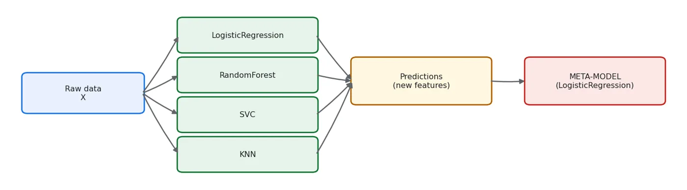
Stacking: the base models' predictions serve as features for the meta-model.
stack = StackingClassifier(
    estimators=[(n, pipe(m)) for n, m in bases.items()],
    final_estimator=LogisticRegression(max_iter=3000),
    cv=5,
)
b_stack = cross_val_score(stack, X, y, cv=5, scoring="f1")
print(f"{'method':<30} {'CV F1':>9} {'±':>8}")
print("-" * 50)
print(f"{'Best single model':<30} {best_base[1].mean():>9.4f} {best_base[1].std():>8.4f}")
print(f"{'Voting (soft)':<30} {cross_val_score(soft, X, y, cv=5, scoring='f1').mean():>9.4f}")
print(f"{'Stacking':<30} {b_stack.mean():>9.4f} {b_stack.std():>8.4f}")
method                             CV F1        ±
--------------------------------------------------
Best single model                 0.7299   0.0054
Voting (soft)                     0.7321
Stacking                          0.7290   0.0105
The OOF rule: the heart of stacking
Stacking has one subtle spot, and it's the most confusing form of leakage.
The meta-model learns from the base models' predictions. But on which data should the base models predict?
show(pd.DataFrame([
    {"Way": "The base model predicts on TRAIN", "What happens": "The predictions are too good (the model saw those rows)",
     "Result": "The meta-model is fooled -> LEAKAGE"},
    {"Way": "Out-of-fold (OOF) prediction", "What happens": "Each row's prediction comes from a model that DIDN'T see it",
     "Result": "CORRECT"},
]))
print()
print("sklearn's StackingClassifier(cv=5) does this AUTOMATICALLY.")
print("If you write it by hand, you must use cross_val_predict.")
sklearn's StackingClassifier(cv=5) does this AUTOMATICALLY.
If you write it by hand, you must use cross_val_predict.
| Way | What happens | Result |
|---|---|---|
| The base model predicts on TRAIN | The predictions are too good (the model saw those rows) | The meta-model is fooled -> LEAKAGE |
| Out-of-fold (OOF) prediction | Each row's prediction comes from a model that DIDN'T see it | CORRECT |
# Let me show the WRONG way, by hand, with leakage
X_tr, X_te, y_tr, y_te = train_test_split(X, y, test_size=0.3, random_state=42, stratify=y)
from sklearn.metrics import f1_score

# bad: the base models predict on TRAIN
bad_feat_tr, bad_feat_te = [], []
for name, m in bases.items():
    q = pipe(m).fit(X_tr, y_tr)
    bad_feat_tr.append(q.predict_proba(X_tr)[:, 1])
    bad_feat_te.append(q.predict_proba(X_te)[:, 1])
meta_bad = LogisticRegression(max_iter=3000).fit(np.column_stack(bad_feat_tr), y_tr)
f1_bad = f1_score(y_te, meta_bad.predict(np.column_stack(bad_feat_te)))

# good: OOF predictions
from sklearn.model_selection import cross_val_predict
good_feat_tr, good_feat_te = [], []
for name, m in bases.items():
    oof = cross_val_predict(pipe(m), X_tr, y_tr, cv=5, method="predict_proba")[:, 1]
    good_feat_tr.append(oof)
    good_feat_te.append(pipe(m).fit(X_tr, y_tr).predict_proba(X_te)[:, 1])
meta_good = LogisticRegression(max_iter=3000).fit(np.column_stack(good_feat_tr), y_tr)
f1_good = f1_score(y_te, meta_good.predict(np.column_stack(good_feat_te)))

print(f"Meta-model trained on TRAIN predictions (leakage): test F1 = {f1_bad:.4f}")
print(f"Meta-model trained on OOF predictions (correct)  : test F1 = {f1_good:.4f}")
print(f"sklearn StackingClassifier (OOF automatically)   : test F1 = {f1_score(y_te, stack.fit(X_tr, y_tr).predict(X_te)):.4f}")
Meta-model trained on TRAIN predictions (leakage): test F1 = 0.7466
Meta-model trained on OOF predictions (correct)  : test F1 = 0.7798
sklearn StackingClassifier (OOF automatically)   : test F1 = 0.7798
Look at the results carefully: they're not what you'd expect.
The meta-model trained with leakage gave 0.7466 on test, while the correct OOF version gave 0.7798. In other words, leakage didn't raise the result, it lowered it.
This is a second, less familiar form of leakage. In the Chapter 6 examples, leakage artificially raises the CV score and fools you. Something else happened here:
the base models memorised the training rows, so their train predictions are almost perfect. The meta-model learned to trust those perfect predictions. Then on test, the base models' predictions came out at ordinary quality, and the meta-model, trusting them too much, got things wrong.
So here the leakage broke the model itself. Either way the conclusion is the same: OOF is mandatory.
Leakage doesn't always raise the score
Students remember leakage as "the result looks good but it's a lie". The measurement above shows that sometimes leakage makes the result worse.
So detect leakage from the structure, not from the sign "the score is suspiciously high": "will I have this at prediction time?" and "has this model seen this row?"
Look at the meta-model's weights: they tell you something
If the meta-model is a LogisticRegression, its coefficients show how much "trust" each base model gets.
meta = stack.fit(X, y).final_estimator_
weights = pd.DataFrame({
    "base model": list(bases.keys()),
    "meta-model weight": meta.coef_[0].round(3),
    "single CV F1": [round(scores[n].mean(), 4) for n in bases],
}).sort_values("meta-model weight", key=abs, ascending=False)
show(weights)
| base model | meta-model weight | single CV F1 |
|---|---|---|
| LogisticRegression | 2.137 | 0.727 |
| RandomForest | 1.08 | 0.7 |
| KNN | 0.486 | 0.7 |
| GaussianNB | 0.421 | 0.73 |
| SVC | 0.352 | 0.726 |
Read the table: which model does the meta-model trust most? Not always the best single model: sometimes it gives more weight to a model that differs from the others, because that one adds new information.
Blending: simpler, but more expensive
# blending: the meta-model is trained on a separate hold-out set
X_b_tr, X_blend, y_b_tr, y_blend = train_test_split(X_tr, y_tr, test_size=0.3,
                                                    random_state=42, stratify=y_tr)
bl_tr, bl_te = [], []
for name, m in bases.items():
    q = pipe(m).fit(X_b_tr, y_b_tr)
    bl_tr.append(q.predict_proba(X_blend)[:, 1])
    bl_te.append(q.predict_proba(X_te)[:, 1])
meta_bl = LogisticRegression(max_iter=3000).fit(np.column_stack(bl_tr), y_blend)
print(f"Blending test F1  : {f1_score(y_te, meta_bl.predict(np.column_stack(bl_te))):.4f}")
print(f"Stacking test F1  : {f1_good:.4f}")
print()
print(f"In blending the meta-model was trained on only {len(y_blend)} rows")
print(f"In stacking, on                               {len(y_tr)} rows (via OOF)")
Blending test F1  : 0.7717
Stacking test F1  : 0.7798

In blending the meta-model was trained on only 252 rows
In stacking, on                               840 rows (via OOF)
Blending is easier to understand, but it spends data: the hold-out part isn't used to train the base models.
Cost and benefit
import time
print(f"{'method':<26} {'CV F1':>9} {'training time':>16} {'number of models':>17}")
print("-" * 72)
for name, m, n_model in [
    ("Single LogisticRegression", pipe(LogisticRegression(max_iter=3000)), 1),
    (f"Single {best_base[0]}", pipe(bases[best_base[0]]), 1),
    ("Voting (soft)", soft, 5),
    ("Stacking", stack, 5 * 5 + 1),
]:
    t0 = time.perf_counter()
    b = cross_val_score(m, X, y, cv=5, scoring="f1")
    dt = time.perf_counter() - t0
    print(f"{name:<26} {b.mean():>9.4f} {dt:>15.1f}s {n_model:>17}")
method                         CV F1    training time  number of models
------------------------------------------------------------------------
Single LogisticRegression     0.7273             0.0s                 1
Single GaussianNB             0.7299             0.0s                 1
Voting (soft)                 0.7321             1.3s                 5
Stacking                      0.7290             6.8s                26
Putting an ensemble into production is expensive
With stacking, six models sit on the server and all of them run for every request. Latency goes up 5-6 times (see Chapter 29 of the MLOps book).
So the practical rule is:
- A Kaggle competition -> stacking is used, because even 0.001 matters
- Production -> usually a single model, because maintenance and latency matter more
If the ensemble's gain is within the spread, take the single model. The Chapter 10 rule applies here too.
The final comparison
everything = []
for name in bases:
    everything.append({"model": f"single: {name}", "CV F1": round(scores[name].mean(), 4),
                       "±": round(scores[name].std(), 4)})
for name, m in [("Voting (hard)", hard), ("Voting (soft)", soft), ("Stacking", stack)]:
    b = cross_val_score(m, X, y, cv=5, scoring="f1")
    everything.append({"model": f"ensemble: {name}", "CV F1": round(b.mean(), 4), "±": round(b.std(), 4)})
tab = pd.DataFrame(everything).sort_values("CV F1", ascending=False)
show(tab)
print()
best = tab.iloc[0]
spread = tab["±"].max()
close = tab[tab["CV F1"] > best["CV F1"] - spread]
print(f"Highest: {best['model']} ({best['CV F1']})")
print(f"Within the spread: {len(close)} / {len(tab)} models")
Highest: ensemble: Voting (soft) (0.7321)
Within the spread: 6 / 8 models
| model | CV F1 | ± |
|---|---|---|
| ensemble: Voting (soft) | 0.732 | 0.01 |
| ensemble: Voting (hard) | 0.731 | 0.016 |
| single: GaussianNB | 0.73 | 0.005 |
| ensemble: Stacking | 0.729 | 0.011 |
| single: LogisticRegression | 0.727 | 0.012 |
| single: SVC | 0.726 | 0.013 |
| single: KNN | 0.7 | 0.018 |
| single: RandomForest | 0.7 | 0.014 |
What we learned today
show(pd.DataFrame([
    {"Concept": "Voting", "In one sentence": "A vote or an average; soft is usually better"},
    {"Concept": "Stacking", "In one sentence": "A meta-model learns from the base predictions"},
    {"Concept": "Blending", "In one sentence": "Stacking on a separate hold-out: it spends data"},
    {"Concept": "The OOF rule", "In one sentence": "A meta-model trained on train predictions = LEAKAGE"},
    {"Concept": "The diversity condition", "In one sentence": "The lower the prediction correlation, the bigger the gain"},
    {"Concept": "Meta weights", "In one sentence": "Show which model is trusted"},
    {"Concept": "The cost", "In one sentence": "N models on the server: N times the latency"},
]))
| Concept | In one sentence |
|---|---|
| Voting | A vote or an average; soft is usually better |
| Stacking | A meta-model learns from the base predictions |
| Blending | Stacking on a separate hold-out: it spends data |
| The OOF rule | A meta-model trained on train predictions = LEAKAGE |
| The diversity condition | The lower the prediction correlation, the bigger the gain |
| Meta weights | Show which model is trusted |
| The cost | N models on the server: N times the latency |
Next chapter: the model made a decision. Why did it decide that way?
Questions about this chapter?
The course, homework review and the other five books are in Uzbek. Questions in English are welcome on Telegram.