Error analysis: what to do when the result is bad
The scene: there's a number, now what?
This is where students get stuck most. And most books don't have this chapter.
The model is built. F1 = 0.79. Now what?
A student usually does one of three things:
- Tries another algorithm (XGBoost, then SVM, then a neural network)
- Starts
GridSearchCVand waits - Googles "how to improve model accuracy"
All three are guesses. All three eat time.
The right move is different: open the rows the model got wrong and read them. The data itself tells you what to do.
This is steps 11 and 12 of the protocol.
Column names
The data is synthetic Tashkent rental listings, and its column names are Uzbek. tuman district, xonalar rooms, maydon_m2 area in m², qavat floor, qavatlar_soni floors in the building, metro_km distance to the metro, mebel furnished (0/1), qurilgan_yil year built. The target ijaraga_berildi_30k means rented within 30 days.
Building the model
import pandas as pd
import numpy as np
from sklearn.model_selection import train_test_split
from sklearn.pipeline import Pipeline
from sklearn.compose import ColumnTransformer
from sklearn.preprocessing import StandardScaler, OneHotEncoder
from sklearn.impute import SimpleImputer
from sklearn.linear_model import LogisticRegression
from sklearn.metrics import f1_score, accuracy_score

df = pd.read_csv(DATA / "uy_ijara.csv")
num = ["xonalar", "maydon_m2", "qavat", "qavatlar_soni", "metro_km", "mebel", "qurilgan_yil"]
X, y = df[num + ["tuman"]], df["ijaraga_berildi_30k"]
X_tr, X_te, y_tr, y_te = train_test_split(X, y, test_size=0.3, random_state=42, stratify=y)

pipe = Pipeline([
    ("prep", ColumnTransformer([
        ("num", Pipeline([("impute", SimpleImputer(strategy="median")),
                          ("scale", StandardScaler())]), num),
        ("cat", OneHotEncoder(handle_unknown="ignore"), ["tuman"]),
    ])),
    ("model", LogisticRegression(max_iter=2000)),
]).fit(X_tr, y_tr)

pred = pipe.predict(X_te)
proba = pipe.predict_proba(X_te)[:, 1]
print(f"Accuracy: {accuracy_score(y_te, pred):.4f}")
print(f"F1      : {f1_score(y_te, pred):.4f}")
print()
print("Now we look NOT AT THESE NUMBERS, BUT AT THE MISTAKES.")
Accuracy: 0.7778
F1      : 0.7938

Now we look NOT AT THESE NUMBERS, BUT AT THE MISTAKES.
Step 1. Read the wrong rows with your own eyes
analysis = X_te.copy()
analysis["truth"] = y_te
analysis["pred"] = pred
analysis["confidence"] = proba.round(3)
analysis["wrong"] = (analysis.truth != analysis.pred).astype(int)

print(f"Total mistakes: {analysis.wrong.sum()} / {len(analysis)} ({analysis.wrong.mean():.1%})")
print()
print("The 6 rows the model got wrong MOST CONFIDENTLY:")
worst = analysis[analysis.wrong == 1].assign(
    error=lambda d: (d.confidence - d.truth).abs()).nlargest(6, "error")
show(worst[["tuman", "xonalar", "maydon_m2", "metro_km", "mebel", "truth", "pred", "confidence"]])
Total mistakes: 80 / 360 (22.2%)

The 6 rows the model got wrong MOST CONFIDENTLY:
| tuman | xonalar | maydon_m2 | metro_km | mebel | truth | pred | confidence |
|---|---|---|---|---|---|---|---|
| Shayxontohur | 1 | 29 | 2.78 | 0 | 0 | 1 | 0.855 |
| Sergeli | 2 | 34.7 | 4.45 | 1 | 0 | 1 | 0.85 |
| Chilonzor | 4 | 84.5 | 1.59 | 1 | 1 | 0 | 0.186 |
| Bektemir | 1 | 25.8 | 1.89 | 0 | 0 | 1 | 0.808 |
| Yakkasaroy | 4 | 75 | 1.62 | 1 | 1 | 0 | 0.205 |
| Yunusobod | 1 | 42.1 | 5.58 | 0 | 0 | 1 | 0.772 |
Read this table; don't rush past it. Look at each row and ask yourself: "what would I say about this flat?"
If you'd get it wrong too, the data doesn't hold enough information (you need a new column). If you'd get it right, the model needs a new view of the data to see what you see.
Step 2. Count the mistakes by group
Reading by eye is the first step. Then we check with numbers: are the mistakes concentrated in one place?
def slice_by(col, label=None):
    g = analysis.groupby(col, observed=True).agg(total=("wrong", "size"), wrong=("wrong", "sum"))
    g["error_rate"] = (g.wrong / g.total).round(3)
    g = g[g.total >= 10].sort_values("error_rate", ascending=False)
    print(f"--- by {label or col} ---")
    print(g.to_string())
    print()

slice_by("tuman")
slice_by("xonalar")
--- by tuman ---
                total  wrong  error_rate
tuman
Shayxontohur       38     12       0.316
Mirzo Ulug'bek     49     13       0.265
Olmazor            46     11       0.239
Yakkasaroy         27      6       0.222
Yunusobod          59     13       0.220
Bektemir           27      5       0.185
Chilonzor          67     12       0.179
Sergeli            47      8       0.170

--- by xonalar ---
         total  wrong  error_rate
xonalar
2          134     45       0.336
3           97     25       0.258
4           52      5       0.096
1           62      5       0.081
5           15      0       0.000
This is the heart of error analysis. The overall error rate is one number, but across groups it is not evenly spread.
Let's group the numeric columns too, cutting them into bins first.
analysis["area_bin"] = pd.cut(analysis.maydon_m2, bins=[0, 40, 60, 80, 300],
                              labels=["<40", "40-60", "60-80", "80+"])
analysis["metro_bin"] = pd.cut(analysis.metro_km, bins=[0, 1, 2.5, 5, 20],
                               labels=["<1km", "1-2.5km", "2.5-5km", "5km+"])
slice_by("area_bin", "area")
slice_by("metro_bin", "distance to metro")
--- by area ---
          total  wrong  error_rate
area_bin
40-60       149     50       0.336
60-80        91     19       0.209
<40          73      9       0.123
80+          47      2       0.043

--- by distance to metro ---
           total  wrong  error_rate
metro_bin
5km+          31      8       0.258
2.5-5km      173     43       0.249
1-2.5km      103     23       0.223
<1km          53      6       0.113
Step 3. Look at the two kinds of mistake separately
FP and FN are two different diseases. Analysing them together is treating two patients with one pill.
fp = analysis[(analysis.truth == 0) & (analysis.pred == 1)]
fn = analysis[(analysis.truth == 1) & (analysis.pred == 0)]

print(f"FP (said yes, was no): {len(fp)}")
print(f"FN (said no, was yes): {len(fn)}")
print()
rows = []
for c in ["maydon_m2", "metro_km", "xonalar", "mebel", "qavat"]:
    rows.append({"Column": c,
                 "FP mean": round(fp[c].mean(), 2),
                 "FN mean": round(fn[c].mean(), 2),
                 "Correct mean": round(analysis[analysis.wrong == 0][c].mean(), 2)})
show(pd.DataFrame(rows))
FP (said yes, was no): 52
FN (said no, was yes): 28
| Column | FP mean | FN mean | Correct mean |
|---|---|---|---|
| maydon_m2 | 47.89 | 65.61 | 57.67 |
| metro_km | 3.04 | 2.99 | 2.75 |
| xonalar | 2.08 | 2.93 | 2.55 |
| mebel | 0.54 | 0.68 | 0.62 |
| qavat | 5.21 | 4.75 | 5.38 |
Read the table column by column. If the FP and FN means differ, that column explains the kind of mistake.
Step 4. The confidence distribution: where is the model unsure
import matplotlib.pyplot as plt

figure, axes = plt.subplots(1, 2, figsize=(13, 4.5))

axes[0].hist([analysis[analysis.truth == 0].confidence, analysis[analysis.truth == 1].confidence],
             bins=20, label=["actually slow", "actually fast"], color=["#c5221f", "#137333"],
             alpha=.75, stacked=False)
axes[0].axvline(0.5, color="k", ls="--", label="threshold 0.5")
axes[0].set_xlabel("Model confidence"); axes[0].set_ylabel("Number of rows")
axes[0].set_title("Confidence distribution"); axes[0].legend(); axes[0].grid(alpha=.3)

bins = pd.cut(analysis.confidence, bins=np.arange(0, 1.01, 0.1))
error_rate = analysis.groupby(bins, observed=True).wrong.mean()
axes[1].bar(range(len(error_rate)), error_rate.values, color="#1a73e8", alpha=.8)
axes[1].set_xticks(range(len(error_rate)))
axes[1].set_xticklabels([f"{i/10:.1f}" for i in range(len(error_rate))], rotation=45)
axes[1].set_xlabel("Confidence bin"); axes[1].set_ylabel("Error rate")
axes[1].set_title("At which confidence does it go wrong most"); axes[1].grid(alpha=.3, axis="y")

fig("xato_tahlili.png", caption="Left: how well the two classes separate by confidence. Right: in which confidence bin the mistakes gather.")
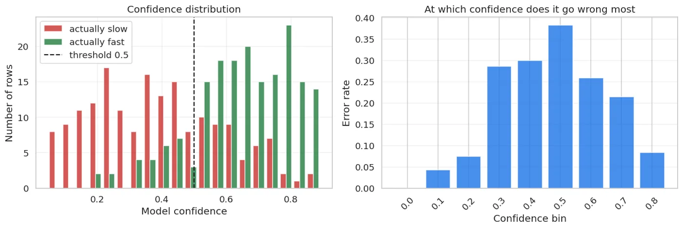
Left: how well the two classes separate by confidence. Right: in which confidence bin the mistakes gather.
The chart on the right matters: the mistakes gather around 0.5. That's normal: the model goes wrong where it is unsure.
But if there are many mistakes around 0.9 too, that's a serious signal. If the model is confidently wrong, the data either has wrong labels or is missing an important column.
Step 5. Do we need more data? Measure it
You can't answer this question by guessing. You have to measure it: a learning curve.
from sklearn.model_selection import learning_curve

sizes, train_scores, val_scores = learning_curve(
    pipe, X, y, train_sizes=np.linspace(0.15, 1.0, 8), cv=5,
    scoring="f1", shuffle=True, random_state=42)

table = pd.DataFrame({
    "train size": sizes,
    "train F1": train_scores.mean(axis=1).round(4),
    "val F1": val_scores.mean(axis=1).round(4),
    "GAP": (train_scores.mean(axis=1) - val_scores.mean(axis=1)).round(4),
})
show(table)
| train size | train F1 | val F1 | GAP |
|---|---|---|---|
| 144 | 0.741 | 0.695 | 0.046 |
| 260 | 0.74 | 0.718 | 0.021 |
| 377 | 0.743 | 0.72 | 0.024 |
| 493 | 0.748 | 0.731 | 0.017 |
| 610 | 0.745 | 0.732 | 0.013 |
| 726 | 0.732 | 0.731 | 0.001 |
| 843 | 0.731 | 0.73 | 0.001 |
| 960 | 0.728 | 0.727 | 0 |
figure2, ax = plt.subplots(figsize=(9, 5))
ax.plot(sizes, train_scores.mean(axis=1), "b-o", lw=2, label="Train F1")
ax.plot(sizes, val_scores.mean(axis=1), "r-o", lw=2, label="Validation F1")
ax.fill_between(sizes, train_scores.mean(axis=1), val_scores.mean(axis=1), alpha=.15, color="red")
ax.set_xlabel("Number of training rows"); ax.set_ylabel("F1")
ax.set_title("Learning curve: would more data help?")
ax.legend(); ax.grid(alpha=.3)
fig("learning_curve.png", caption="When the two lines have come together and flattened, more data won't help.")
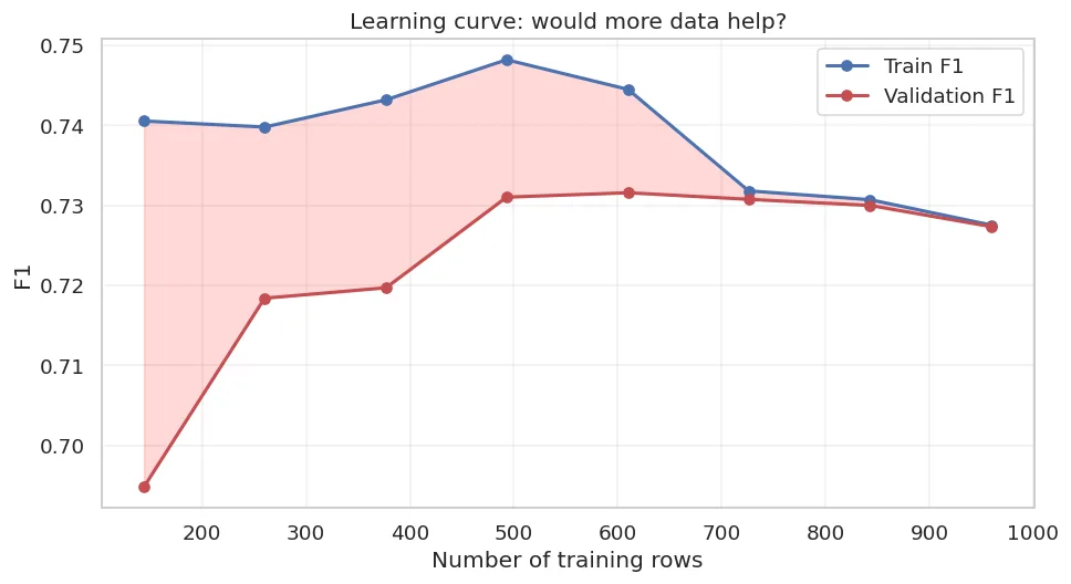
When the two lines have come together and flattened, more data won't help.
How to read the chart:
show(pd.DataFrame([
    {"What you see": "The two lines are CLOSE and both LOW", "Diagnosis": "Underfitting (high bias)",
     "Action": "A stronger model, more features. More DATA WON'T HELP"},
    {"What you see": "Train HIGH, validation LOW, a WIDE gap", "Diagnosis": "Overfitting (high variance)",
     "Action": "More data, regularisation, a simpler model"},
    {"What you see": "Validation is still RISING", "Diagnosis": "Too little data",
     "Action": "Collecting more data HELPS"},
    {"What you see": "Validation has FLATTENED", "Diagnosis": "Enough data",
     "Action": "You need a new column or another model"},
]))
| What you see | Diagnosis | Action |
|---|---|---|
| The two lines are CLOSE and both LOW | Underfitting (high bias) | A stronger model, more features. More DATA WON'T HELP |
| Train HIGH, validation LOW, a WIDE gap | Overfitting (high variance) | More data, regularisation, a simpler model |
| Validation is still RISING | Too little data | Collecting more data HELPS |
| Validation has FLATTENED | Enough data | You need a new column or another model |
last_gap = train_scores.mean(axis=1)[-1] - val_scores.mean(axis=1)[-1]
last_rise = val_scores.mean(axis=1)[-1] - val_scores.mean(axis=1)[-3]
print(f"GAP at the last point         : {last_gap:.4f}")
print(f"Latest rise in validation     : {last_rise:+.4f}")
print()
if last_gap > 0.08:
    print("DIAGNOSIS: signs of overfitting -> more data or regularisation")
elif last_rise > 0.01:
    print("DIAGNOSIS: validation is still rising -> more data HELPS")
else:
    print("DIAGNOSIS: enough data, the lines are close -> you need a NEW COLUMN or another model")
GAP at the last point         : 0.0002
Latest rise in validation     : -0.0034

DIAGNOSIS: enough data, the lines are close -> you need a NEW COLUMN or another model
Step 6. A decision and one change
Now you have evidence. From the table you pick one action.
show(pd.DataFrame([
    {"Evidence": "The mistakes cluster in one group", "Action": "A new column for that group, or a separate model"},
    {"Evidence": "The FP and FN means differ", "Action": "Move the threshold (Chapter 9)"},
    {"Evidence": "The model is confidently wrong", "Action": "Check the labels, add the important column"},
    {"Evidence": "Learning curve: validation is rising", "Action": "Collect more data"},
    {"Evidence": "Learning curve: the GAP is wide", "Action": "Regularisation or a simpler model"},
    {"Evidence": "Learning curve: both low and flat", "Action": "A stronger model (tree, boosting)"},
    {"Evidence": "No evidence, everything is normal", "Action": "Stop. The model is good enough (Chapter 40)"},
]))
| Evidence | Action |
|---|---|
| The mistakes cluster in one group | A new column for that group, or a separate model |
| The FP and FN means differ | Move the threshold (Chapter 9) |
| The model is confidently wrong | Check the labels, add the important column |
| Learning curve: validation is rising | Collect more data |
| Learning curve: the GAP is wide | Regularisation or a simpler model |
| Learning curve: both low and flat | A stronger model (tree, boosting) |
| No evidence, everything is normal | Stop. The model is good enough (Chapter 40) |
What does the evidence say in our case? The learning curve gave its diagnosis. Let's try exactly that action: check whether a linear model isn't enough.
from sklearn.ensemble import RandomForestClassifier
from sklearn.model_selection import cross_val_score

def with_pipe(model):
    return Pipeline([
        ("prep", ColumnTransformer([
            ("num", Pipeline([("impute", SimpleImputer(strategy="median")),
                              ("scale", StandardScaler())]), num),
            ("cat", OneHotEncoder(handle_unknown="ignore"), ["tuman"]),
        ])),
        ("model", model),
    ])

lr = cross_val_score(with_pipe(LogisticRegression(max_iter=2000)), X, y, cv=5, scoring="f1")
rf = cross_val_score(with_pipe(RandomForestClassifier(n_estimators=200, random_state=42)),
                     X, y, cv=5, scoring="f1")
print(f"Logistic Regression: {lr.mean():.4f} ±{lr.std():.4f}")
print(f"Random Forest      : {rf.mean():.4f} ±{rf.std():.4f}")
print(f"Gap                : {rf.mean() - lr.mean():+.4f}  (spread ±{max(lr.std(), rf.std()):.4f})")
print()
print("Verdict:", "Random Forest is reliably better" if rf.mean() - lr.mean() > max(lr.std(), rf.std())
      else "The gap is within the spread: keep the simpler model")
Logistic Regression: 0.7273 ±0.0118
Random Forest      : 0.6998 ±0.0138
Gap                : -0.0275  (spread ±0.0138)

Verdict: The gap is within the spread: keep the simpler model
ONE change at a time
If you add a new column, change the model and move the threshold all at once, and the result improves, you don't know which one helped.
Next time you apply that "good recipe" on another project and it doesn't work, because you never knew what worked.
One change -> measure -> write it down -> the next one.
The error-analysis notebook
Write down every loop. This notebook is your most valuable document.
notebook = """
+----------------------------------------------------------------------+
|  ERROR-ANALYSIS NOTEBOOK                                             |
+----------------------------------------------------------------------+
|  Date        :                                                       |
|  Model       :                                                       |
|  Metric      : F1 = ______  (CV: ______ +- ______)                   |
|  Baseline    : ______                                                |
+----------------------------------------------------------------------+
|  1. Which group do the mistakes cluster in?                          |
|     ................................................................ |
|  2. How do FP and FN differ?                                         |
|     ................................................................ |
|  3. Is the model confidently wrong? (mistakes at 0.9+)               |
|     ................................................................ |
|  4. Learning curve diagnosis?                                        |
|     [ ] underfitting  [ ] overfitting  [ ] too little data  [ ] ok   |
+----------------------------------------------------------------------+
|  DECISION (ONLY ONE):                                                |
|     [ ] new feature: ..............................................  |
|     [ ] another model: ............................................  |
|     [ ] more data                                                    |
|     [ ] move the threshold: .......................................  |
|     [ ] stop                                                         |
+----------------------------------------------------------------------+
|  Result: ______  (previous: ______)   Gap: ______                    |
|  Was my hypothesis right?  [ ] yes   [ ] NO <- the most valuable     |
+----------------------------------------------------------------------+
"""
print(notebook)
+----------------------------------------------------------------------+
|  ERROR-ANALYSIS NOTEBOOK                                             |
+----------------------------------------------------------------------+
|  Date        :                                                       |
|  Model       :                                                       |
|  Metric      : F1 = ______  (CV: ______ +- ______)                   |
|  Baseline    : ______                                                |
+----------------------------------------------------------------------+
|  1. Which group do the mistakes cluster in?                          |
|     ................................................................ |
|  2. How do FP and FN differ?                                         |
|     ................................................................ |
|  3. Is the model confidently wrong? (mistakes at 0.9+)               |
|     ................................................................ |
|  4. Learning curve diagnosis?                                        |
|     [ ] underfitting  [ ] overfitting  [ ] too little data  [ ] ok   |
+----------------------------------------------------------------------+
|  DECISION (ONLY ONE):                                                |
|     [ ] new feature: ..............................................  |
|     [ ] another model: ............................................  |
|     [ ] more data                                                    |
|     [ ] move the threshold: .......................................  |
|     [ ] stop                                                         |
+----------------------------------------------------------------------+
|  Result: ______  (previous: ______)   Gap: ______                    |
|  Was my hypothesis right?  [ ] yes   [ ] NO <- the most valuable     |
+----------------------------------------------------------------------+
Pay special attention to the last line. A rejected hypothesis is the most valuable entry. It tells you that your assumptions about your data were wrong, and no book can give you that knowledge.
What we learned today
show(pd.DataFrame([
    {"Step": "1. Read the mistakes", "Tool": "nlargest(confidence), with your own eyes"},
    {"Step": "2. Count by group", "Tool": "groupby(column).wrong.mean()"},
    {"Step": "3. Separate FP and FN", "Tool": "Two kinds of mistake, two different causes"},
    {"Step": "4. Confidence distribution", "Tool": "Where the model is unsure, where it is confidently wrong"},
    {"Step": "5. Learning curve", "Tool": "Do you need more data? A MEASUREMENT, not a guess"},
    {"Step": "6. ONE change", "Tool": "An evidence-based decision, then back to step 9"},
]))
| Step | Tool |
|---|---|
| 1. Read the mistakes | nlargest(confidence), with your own eyes |
| 2. Count by group | groupby(column).wrong.mean() |
| 3. Separate FP and FN | Two kinds of mistake, two different causes |
| 4. Confidence distribution | Where the model is unsure, where it is confidently wrong |
| 5. Learning curve | Do you need more data? A MEASUREMENT, not a guess |
| 6. ONE change | An evidence-based decision, then back to step 9 |
That completes Part 2. You can now split the data, know your baseline, choose the metric, move the threshold, get a reliable score with CV, and find the next step with error analysis.
In the three exercises of Chapters 43–45 you do all of this yourself.
Questions about this chapter?
The course, homework review and the other five books are in Uzbek. Questions in English are welcome on Telegram.