A new dataset: 12 steps
The book is complete: 48 chapters
Every chapter is written: 1–48. Every number comes from code that build.py executed. There is no number typed in by hand or guessed.
| Part | Chapters | Topic |
|---|---|---|
| 0 | 1 | A new dataset: the 12-step protocol |
| 1 | 2–5 | What ML is · SQL · visualisation · data preparation |
| 2 | 6–11 | Split and leakage · baseline · metrics · ROC/PR · CV · error analysis |
| 3 | 12–14 | Vectors and matrices · gradient descent · the normal equation |
| 4 | 15–22 | Linear · logistic · regularisation · tree · forest · boosting · KNN/Bayes · SVM |
| 5 | 23–26 | Feature engineering · tuning · stacking · SHAP |
| 6 | 27–29 | PCA · clustering · LDA |
| 7 | 30–36 | Neural networks · backprop · Keras · PyTorch · CNN · RNN/LSTM · attention |
| 8 | 37–41 | The chain: data collection → dataset → fine-tuning → saving → Django API |
| 9 | 42–45 | Walking through without edits · three independent exercises |
| Appendix | 46–48 | Confusion-solver · interview questions · cheat sheet |
Where to start:
- If you have a new dataset in hand: this chapter (1), then Chapter 42.
- If you want to strengthen the theory: from Chapter 2 in order.
- If some concept is confusing: Chapter 46.
- If you want to run the project: Part 8 (37–41).
The datasets: which are real, which are synthetic
This has to be honest, because the whole book rests on measured numbers.
| File | Kind | Note |
|---|---|---|
uy_ijara.csv |
synthetic | Built by datasets/generate.py with a fixed seed. Traps were planted in it ON PURPOSE |
talaba_bitirdi.csv |
synthetic | From the same generator, with hidden leakage (Chapter 45) |
titanic.csv |
real | The Kaggle/seaborn dataset |
penguins.csv |
real | Palmer Penguins |
iflos_savdo.csv |
real and dirty | From the Data Analytics course, left uncleaned |
Synthetic data is not a bad thing. It is reproducible: you, I and your students all see exactly the same numbers. In real datasets nobody invented the traps; they are simply there.
When you copy the code: what DATA is
Every block in the book reads like this:
df = pd.read_csv(DATA / "uy_ijara.csv")
DATA is a folder path the book provides automatically when it is built. If you copy the code, you won't have it and you'll get a NameError.
The fix is one line at the top of your file:
from pathlib import Path

DATA = Path("datasets")      # if the CSV files are in a `datasets` folder
# DATA = Path(".")           # if the CSV files are in the SAME folder as the code

ISH = Path("ish")            # Chapters 37-41 write their project files here
ISH.mkdir(exist_ok=True)
ISH is the project folder for Part 8 (Chapters 37–41). The book writes the scraper, the cleaning and the API files there. Other chapters don't need it.
After that, every block in the book runs unchanged.
Libraries you need:
pip install pandas numpy scikit-learn matplotlib seaborn
Column names
The main dataset is synthetic Tashkent rental listings, and its column names are Uzbek. elon_id listing id, tuman district, xonalar rooms, maydon_m2 area in m², qavat floor, qavatlar_soni floors in the building, metro_km distance to the metro, mebel furnished (0/1), qurilgan_yil year built, narx_matn price as text, agent_komissiyasi agent fee, narx_usd monthly rent in USD, ijaraga_berildi_30k rented within 30 days.
A familiar situation
It's 9 pm. You're at your computer. You just downloaded a new file from Kaggle: uy_ijara.csv.
You open it. 1200 rows, 13 columns. You look at the screen.
And... you freeze.
Where do you start? Which column matters? Can I just call LogisticRegression? Which column am I predicting? If I get a result, how do I know it's any good?
This is not your fault. In class you were always handed a ready-made X and y. Nobody ever gave you a single CSV file and said "here, get to work". You learned algorithms, but you never learned the job.
This chapter fixes that.
Why even programmers freeze
Let's compare.
Someone learning to drive learns two different things:
- Mechanics: accelerator, brake, gears, steering.
- Procedure: you get in the car, then what first? Seatbelt. Then the mirror. Then the rear view. Then the engine. Then the gear.
Someone who knows the mechanics but not the procedure sits in the car and freezes. They know the accelerator and the brake, but they don't know what to do first.
ML is exactly the same. You know fit() and predict(). Those are the accelerator and the brake. But there's no procedure.
Here is the procedure. Twelve steps. Each step answers one question and produces one decision.
How to use this chapter
Read it once. Then print the card on the last page and put it on your desk. When you see a new dataset, read the card; don't think. After a month or two you won't need the card.
The protocol: 12 steps
import pandas as pd
show(pd.DataFrame([
    {"Step": 1,  "What I do": "Open the file", "The decision it produces": "How many rows, how many columns; I write it down"},
    {"Step": 2,  "What I do": "Name the target", "The decision it produces": "One sentence: what I predict from what"},
    {"Step": 3,  "What I do": "Look at the target's type", "The decision it produces": "Regression / classification / clustering"},
    {"Step": 4,  "What I do": "COUNT the target", "The decision it produces": "Is it imbalanced? What is my baseline?"},
    {"Step": 5,  "What I do": "Split NOW", "The decision it produces": "The test set gets locked away"},
    {"Step": 6,  "What I do": "Dummy model", "The decision it produces": "The pass mark, as a single number"},
    {"Step": 7,  "What I do": "Find the poisonous columns", "The decision it produces": "A list of columns to drop"},
    {"Step": 8,  "What I do": "Missing values and types", "The decision it produces": "For each column: fill or drop"},
    {"Step": 9,  "What I do": "One simple model in a Pipeline", "The decision it produces": "Is it better than the dummy?"},
    {"Step": 10, "What I do": "Choose the metric", "The decision it produces": "Which number I judge by"},
    {"Step": 11, "What I do": "READ the rows it got wrong", "The decision it produces": "What the model doesn't understand"},
    {"Step": 12, "What I do": "Make a decision", "The decision it produces": "One change, then back to step 9"},
]))
| Step | What I do | The decision it produces |
|---|---|---|
| 1 | Open the file | How many rows, how many columns; I write it down |
| 2 | Name the target | One sentence: what I predict from what |
| 3 | Look at the target's type | Regression / classification / clustering |
| 4 | COUNT the target | Is it imbalanced? What is my baseline? |
| 5 | Split NOW | The test set gets locked away |
| 6 | Dummy model | The pass mark, as a single number |
| 7 | Find the poisonous columns | A list of columns to drop |
| 8 | Missing values and types | For each column: fill or drop |
| 9 | One simple model in a Pipeline | Is it better than the dummy? |
| 10 | Choose the metric | Which number I judge by |
| 11 | READ the rows it got wrong | What the model doesn't understand |
| 12 | Make a decision | One change, then back to step 9 |
Now let's walk through those twelve steps on a real file, one by one. Every number comes from executed code.
Step 1. Open the file
The first three commands. Always these three.
import pandas as pd

df = pd.read_csv(DATA / "uy_ijara.csv")

print("shape:", df.shape)
print()
print(df.dtypes.to_string())
shape: (1200, 13)

elon_id                 object
tuman                   object
xonalar                  int64
maydon_m2              float64
qavat                    int64
qavatlar_soni            int64
metro_km               float64
mebel                    int64
qurilgan_yil           float64
narx_matn               object
agent_komissiyasi        int64
narx_usd                 int64
ijaraga_berildi_30k      int64
What we saw:
- 1200 rows, 13 columns. A small file. That's good: it runs fast and we find mistakes fast.
tuman,elon_id,narx_matnare object, meaning text.- The rest are numbers.
Notice: narx_matn is text. But it has "narx" (price) in its name, so it should have been a number. First suspicion. We come back to it in step 7.
Now let's look at the rows themselves. Working without looking at the table is like driving with your eyes closed.
show(df.head(6))
| elon_id | tuman | xonalar | maydon_m2 | qavat | qavatlar_soni | metro_km | mebel | qurilgan_yil | narx_matn | agent_komissiyasi | narx_usd | ijaraga_berildi_30k |
|---|---|---|---|---|---|---|---|---|---|---|---|---|
| UZ-100000 | Chilonzor | 2 | 40.6 | 2 | 14 | 1.43 | 1 | 2 016 | 9 500 000 so'm | 0 | 760 | 0 |
| UZ-100001 | Yakkasaroy | 2 | 55.5 | 1 | 2 | 4.18 | 1 | 1 977 | 6 875 000 so'm | 0 | 550 | 0 |
| UZ-100002 | Mirzo Ulug'bek | 5 | 114 | 2 | 4 | 3.84 | 1 | 2 010 | 17 687 500 so'm | 0 | 1 415 | 0 |
| UZ-100003 | Mirzo Ulug'bek | 3 | 72.1 | 3 | 4 | 2.99 | 1 | 2 007 | 12 312 500 so'm | 0 | 985 | 0 |
| UZ-100004 | Chilonzor | 2 | 46.4 | 2 | 2 | 4.58 | 0 | 1 989 | 6 875 000 so'm | 275 | 550 | 1 |
| UZ-100005 | Olmazor | 3 | 61 | 9 | 11 | 1.9 | 0 | 1 987 | 7 750 000 so'm | 310 | 620 | 1 |
Don't skip df.head()
I have watched many students go straight from read_csv to fit(). Then they spend an hour hunting for an error. One look at head() shows that narx_matn is text and that elon_id is useless. One second saves an hour.
Step 2. Name the target
There is no code in this step. You write one sentence.
"I predict whether a flat is rented within 30 days from its features."
Don't move on until you have written that sentence. If you can't write it, you haven't understood the problem, and no model will help.
This file has two possible targets:
| Column | Meaning | Task |
|---|---|---|
narx_usd |
Monthly rent | predict a number |
ijaraga_berildi_30k |
Was it rented within 30 days | predict yes/no |
We take the second one. The first one comes in Chapter 15.
Why this question
"Will this flat be rented quickly?" is a real business question. If the agency knows the answer, it can fix the price in advance. If your question helps nobody, building a model is a waste of time.
Step 3. Look at the target's type
print("ijaraga_berildi_30k:")
print("  dtype         :", df.ijaraga_berildi_30k.dtype)
print("  unique values :", sorted(df.ijaraga_berildi_30k.unique().tolist()))
print()
print("narx_usd:")
print("  dtype         :", df.narx_usd.dtype)
print("  unique values :", df.narx_usd.nunique())
ijaraga_berildi_30k:
  dtype         : int64
  unique values : [0, 1]

narx_usd:
  dtype         : int64
  unique values : 207
The rule is very simple:
show(pd.DataFrame([
    {"What the target looks like": "Two values (0/1, yes/no)", "Task": "Binary classification"},
    {"What the target looks like": "A few labels (3-10 kinds)", "Task": "Multiclass classification"},
    {"What the target looks like": "A continuous number (price, temperature, time)", "Task": "Regression"},
    {"What the target looks like": "NO target", "Task": "Clustering or PCA"},
]))
| What the target looks like | Task |
|---|---|
| Two values (0/1, yes/no) | Binary classification |
| A few labels (3-10 kinds) | Multiclass classification |
| A continuous number (price, temperature, time) | Regression |
| NO target | Clustering or PCA |
We have [0, 1]: two values. So it's binary classification. Decision made.
narx_usd has 207 different values. It's a continuous number, so it would be regression.
Step 4. COUNT the target
This is the step people skip most often. And the one that costs the most.
ratio = df.ijaraga_berildi_30k.value_counts(normalize=True).sort_index()
print("0 (not rented):", f"{ratio[0]:.1%}")
print("1 (rented)    :", f"{ratio[1]:.1%}")
print()
print("If the model says '1' to EVERYONE, accuracy =", f"{ratio[1]:.1%}")
0 (not rented): 49.3%
1 (rented)    : 50.7%

If the model says '1' to EVERYONE, accuracy = 50.7%
That number, 50.7%, is your enemy. Why?
Because a model that learned nothing gets that much too. A model that says "every flat gets rented" shows 50.7% accuracy. If you get 52% and feel happy, you fooled yourself.
This dataset is kind. Real data is not.
We have 50/50, which is the comfortable case. Real projects are often 95/5 or 99/1. In fraud detection, fraud is 0.1%. There, a model that says "no" to everyone gets 99.9% accuracy and is completely useless. Chapter 9 looks at exactly that case.
So the rule is: count the target before you look at accuracy.
Step 5. Split NOW
Attention: this step happens now. Before cleaning. Before scaling. Before drawing any chart.
from sklearn.model_selection import train_test_split

X = df.drop(columns=["ijaraga_berildi_30k", "narx_usd"])
y = df["ijaraga_berildi_30k"]

X_tr, X_te, y_tr, y_te = train_test_split(
    X, y, test_size=0.3, random_state=42, stratify=y
)

print(f"train: {len(X_tr)} rows, rented {y_tr.mean():.1%}")
print(f"test : {len(X_te)} rows, rented {y_te.mean():.1%}")
train: 840 rows, rented 50.7%
test : 360 rows, rented 50.6%
What did stratify=y do? It kept the same ratio in train and test: about 50.7% in both. Without it, test could have come out at 60% by chance, and your results would be a lie.
Why now? Because later you'll use StandardScaler. If you fit the scaler on all the data, it "sees" the mean and standard deviation of the test set. The model will have seen the exam questions in advance. The result looks great, and it collapses on the server.
The most expensive mistake in this book
This is data leakage. The most dangerous thing about it: it raises no error. The code runs, the number looks good, you are happy. The problem shows up a month later, when you put the model into production.
The rule: the test set is locked in a safe. You look at it once, at the very end.
Step 6. The dummy model: the pass mark
Now you build your first "model". It learns nothing. It just says the most common answer.
Why do you need it? Because you need a point of comparison. Without a thermometer, the word "hot" means nothing.
from sklearn.dummy import DummyClassifier
from sklearn.metrics import accuracy_score

dummy = DummyClassifier(strategy="most_frequent").fit(X_tr[["xonalar"]], y_tr)
baseline = accuracy_score(y_te, dummy.predict(X_te[["xonalar"]]))

print(f"BASELINE (a model that learned nothing): {baseline:.4f}")
print()
print("Write this number down. Your model MUST beat it.")
BASELINE (a model that learned nothing): 0.5056

Write this number down. Your model MUST beat it.
0.5056. Written down. Now we have a pass mark.
This step is one line of code. But it saves you from the most common self-deception: "accuracy 85%, great!" when the target is 85% one class.
Step 7. Find the poisonous columns
Now we check the columns one by one. There are three kinds of poison.
Poison 1: a different value in every row
print("Unique values per column (out of 1200 rows):")
for col in X_tr.columns:
    n = X_tr[col].nunique()
    flag = "   <-- SUSPICIOUS: different in almost every row" if n > len(X_tr) * 0.9 else ""
    print(f"  {col:22s} {n:5d}{flag}")
Unique values per column (out of 1200 rows):
  elon_id                  840   <-- SUSPICIOUS: different in almost every row
  tuman                      8
  xonalar                    5
  maydon_m2                521
  qavat                     16
  qavatlar_soni             15
  metro_km                 440
  mebel                      2
  qurilgan_yil              50
  narx_matn                193
  agent_komissiyasi         83
elon_id has 840 different values in 840 rows. It is an identifier, not a feature. It explains nothing.
Why is it dangerous? A tree model memorises every ID and scores 100% on train. When a new listing arrives, its ID isn't in the tree, and the model doesn't know what to do.
Rule: IDs, codes, phone numbers, passport numbers get dropped.
Poison 2: should be a number, but it's text
print("first 3 values of narx_matn:")
for v in X_tr.narx_matn.head(3):
    print("  ", repr(v))
print()
print("dtype:", X_tr.narx_matn.dtype, "<-- object = text")
first 3 values of narx_matn:
   "12 125 000 so'm"
   "10 625 000 so'm"
   "11 687 500 so'm"

dtype: object <-- object = text
"9 500 000 so'm" is a number (so'm is the Uzbek currency), but pandas read it as text: it contains spaces and the word "so'm".
There are two options: clean it into a number, or drop it. But careful: narx_matn is really just another form of narx_usd, meaning the second target. It must not be used as a feature.
Poison 3: the most dangerous one, leakage
check = X_tr.assign(rented=y_tr).groupby("rented").agent_komissiyasi.agg(["mean", "min", "max"])
show(check.reset_index())
| rented | mean | min | max |
|---|---|---|---|
| 0 | 0 | 0 | 0 |
| 1 | 335.775 | 110 | 610 |
Look. When rented = 0, the fee is always 0. When rented = 1, it is always above zero.
The reason is simple: the agent takes the fee AFTER the flat is rented. At prediction time this column doesn't exist yet.
What happens if we give it to the model? Let me show you.
from sklearn.linear_model import LogisticRegression
from sklearn.metrics import accuracy_score

honest = ["xonalar", "maydon_m2", "qavat", "qavatlar_soni", "metro_km", "mebel"]

m_honest = LogisticRegression(max_iter=2000).fit(X_tr[honest], y_tr)
m_leak = LogisticRegression(max_iter=2000).fit(X_tr[honest + ["agent_komissiyasi"]], y_tr)

acc_honest = accuracy_score(y_te, m_honest.predict(X_te[honest]))
acc_leak = accuracy_score(y_te, m_leak.predict(X_te[honest + ["agent_komissiyasi"]]))

print(f"Honest features         : {acc_honest:.4f}")
print(f"+ agent_komissiyasi     : {acc_leak:.4f}   <-- PERFECT")
Honest features         : 0.7778
+ agent_komissiyasi     : 1.0000   <-- PERFECT
1.0000. One hundred percent. A model that never makes a mistake.
If you see that and feel happy, you just fooled yourself. The model learned nothing. It was simply looking at the answer: "there's a fee, so it was rented."
Put this model on a server and it falls over on the first real request, because a new listing has no fee column.
A perfect result is not a celebration, it's a signal
If accuracy goes above 0.99, your first thought should not be "great model". It should be: "which column is telling it the answer?"
How to check: group each feature by the target (like the groupby above). If one column separates the target completely, it is leakage.
The question: "will I have this column at prediction time?" If not, drop it.
So the columns to drop are:
dropped = {
    "elon_id": "identifier, different in every row",
    "narx_matn": "the text form of the second target",
    "agent_komissiyasi": "LEAKAGE, only known after renting",
}
show(pd.DataFrame([{"Column": k, "Why it is dropped": v} for k, v in dropped.items()]))
| Column | Why it is dropped |
|---|---|
| elon_id | identifier, different in every row |
| narx_matn | the text form of the second target |
| agent_komissiyasi | LEAKAGE, only known after renting |
Step 8. Missing values and types
missing = X_tr.isna().sum()
missing = missing[missing > 0]
if len(missing):
    print("There are missing values:")
    for col, n in missing.items():
        print(f"  {col:16s} {n:3d} ({n/len(X_tr):.1%})")
else:
    print("No missing values")
print()
print("Text columns (need encoding):")
for c in X_tr.select_dtypes("object").columns:
    print(f"  {c:16s} {X_tr[c].nunique()} distinct values")
There are missing values:
  qurilgan_yil       5 (0.6%)

Text columns (need encoding):
  elon_id          840 distinct values
  tuman            8 distinct values
  narx_matn        193 distinct values
qurilgan_yil is missing in 5 rows of the train set (0.6%). That's few. There are three options:
| Option | When |
|---|---|
| Drop the row | When it's very rare (< 1%) and you have plenty of data |
| Fill with the mean / median | A numeric column with 5–30% missing |
| A separate "missing" category | When the absence itself means something |
We fill with the median, and we do it inside the Pipeline, because the median must come from train only.
tuman has 8 different text values. The model doesn't understand text; it has to become numbers. But districts have no order (we don't say Chilonzor > Sergeli), so we use OneHotEncoder.
Step 9. One simple model in a Pipeline
Now the first real model. Note that we use a Pipeline. That's not a style choice, it's protection.
from sklearn.pipeline import Pipeline
from sklearn.compose import ColumnTransformer
from sklearn.preprocessing import StandardScaler, OneHotEncoder
from sklearn.impute import SimpleImputer

num = ["xonalar", "maydon_m2", "qavat", "qavatlar_soni", "metro_km", "mebel", "qurilgan_yil"]
cat = ["tuman"]

prep = ColumnTransformer([
    ("num", Pipeline([
        ("impute", SimpleImputer(strategy="median")),
        ("scale", StandardScaler()),
    ]), num),
    ("cat", OneHotEncoder(handle_unknown="ignore"), cat),
])

pipe = Pipeline([
    ("prep", prep),
    ("model", LogisticRegression(max_iter=2000)),
])

pipe.fit(X_tr, y_tr)
acc = accuracy_score(y_te, pipe.predict(X_te))

print(f"BASELINE   : {baseline:.4f}")
print(f"First model: {acc:.4f}")
print(f"Difference : {acc - baseline:+.4f}")
BASELINE   : 0.5056
First model: 0.7778
Difference : +0.2722
0.7778, which is 0.27 above the baseline. The model really did learn something.
Why does Pipeline matter? Three reasons:
- Protection from leakage. When
fit()is called, the imputer and the scaler learn from train only. You can't get it wrong; the structure won't let you. - One object. When you save the model, the preprocessing is saved with it (Chapter 40).
- Cross-validation works correctly. Preprocessing is redone in every fold (Chapter 10).
The one pattern to remember
This pattern repeats through the whole book:
ColumnTransformer (fill + scale for numbers, OneHot for text) → Pipeline → fit.
Swap the model and you only change the last line. Everything else stays the same.
Step 10. Choose the metric
accuracy = 0.7778. Is that enough? Not yet. What is accuracy hiding?
from sklearn.metrics import confusion_matrix, precision_score, recall_score, f1_score

pred = pipe.predict(X_te)
tn, fp, fn, tp = confusion_matrix(y_te, pred).ravel()

print(f"TN={tn}  FP={fp}  FN={fn}  TP={tp}")
print()
print(f"Accuracy : {acc:.4f}")
print(f"Precision: {precision_score(y_te, pred):.4f}  = TP/(TP+FP) = {tp}/({tp}+{fp})")
print(f"Recall   : {recall_score(y_te, pred):.4f}  = TP/(TP+FN) = {tp}/({tp}+{fn})")
print(f"F1       : {f1_score(y_te, pred):.4f}")
TN=126  FP=52  FN=28  TP=154

Accuracy : 0.7778
Precision: 0.7476  = TP/(TP+FP) = 154/(154+52)
Recall   : 0.8462  = TP/(TP+FN) = 154/(154+28)
F1       : 0.7938
Now we see the detail. The model called 206 flats "rents fast" (154 + 52) and was right about 154 of them. It missed 28 flats that went fast; those are the FN.
Which number matters? That's a business decision, not a mathematical one:
| If your problem is | The metric that matters | Why |
|---|---|---|
| You spend money on ads | Precision | Don't spend on empty listings |
| Not missing a single opportunity | Recall | Don't miss a flat that will go fast |
| Both matter | F1 | Balance |
| Classes are very imbalanced | PR-AUC or macro F1 | Accuracy lies (Chapter 9) |
Chapters 8 and 9 are entirely about this.
Step 11. READ the rows it got wrong
This is the step where students get stuck most. A number came out; now what?
The answer: open the rows the model got wrong and read them. By hand. With your own eyes.
proba = pipe.predict_proba(X_te)[:, 1]
analysis = X_te.assign(truth=y_te, pred=pred, confidence=proba.round(3))

wrong = analysis[analysis.truth != analysis.pred]
print(f"Rows it got wrong: {len(wrong)} ({len(wrong)/len(X_te):.1%})")
print()
print("The 5 rows the model got wrong MOST CONFIDENTLY:")
worst = wrong.assign(error=(wrong.confidence - wrong.truth).abs()).nlargest(5, "error")
show(worst[["tuman", "xonalar", "maydon_m2", "metro_km", "mebel", "truth", "pred", "confidence"]])
Rows it got wrong: 80 (22.2%)

The 5 rows the model got wrong MOST CONFIDENTLY:
| tuman | xonalar | maydon_m2 | metro_km | mebel | truth | pred | confidence |
|---|---|---|---|---|---|---|---|
| Shayxontohur | 1 | 29 | 2.78 | 0 | 0 | 1 | 0.855 |
| Sergeli | 2 | 34.7 | 4.45 | 1 | 0 | 1 | 0.85 |
| Chilonzor | 4 | 84.5 | 1.59 | 1 | 1 | 0 | 0.186 |
| Bektemir | 1 | 25.8 | 1.89 | 0 | 0 | 1 | 0.808 |
| Yakkasaroy | 4 | 75 | 1.62 | 1 | 1 | 0 | 0.205 |
Look at this table and ask yourself:
- Are the mistakes concentrated in one district? Then there isn't enough information about that district.
- In large flats? Then the model has few examples of them.
- In unfurnished ones? Then the
mebelcolumn isn't enough.
Let's count where the mistakes cluster:
total = analysis.groupby("tuman").size()
errors = wrong.groupby("tuman").size()
result = pd.DataFrame({"total": total, "errors": errors}).fillna(0)
result["error_rate"] = (result.errors / result.total).round(3)
show(result.sort_values("error_rate", ascending=False).reset_index())
| tuman | total | errors | error_rate |
|---|---|---|---|
| Shayxontohur | 38 | 12 | 0.316 |
| Mirzo Ulug'bek | 49 | 13 | 0.265 |
| Olmazor | 46 | 11 | 0.239 |
| Yakkasaroy | 27 | 6 | 0.222 |
| Yunusobod | 59 | 13 | 0.22 |
| Bektemir | 27 | 5 | 0.185 |
| Chilonzor | 67 | 12 | 0.179 |
| Sergeli | 47 | 8 | 0.17 |
The answer to "what do I do next?" is right here
Many students stop at step 10: there's a number, but no next move. So they do something random: try another model, spin the hyperparameters, google.
The right move: read the rows it got wrong. The data itself tells you what the model doesn't understand. Chapter 11 is entirely about this.
Step 12. Make a decision
Now you have information. You pick one of five paths:
show(pd.DataFrame([
    {"Path": "Add a new feature", "When": "The mistakes cluster in one group",
     "Example": "price/area ratio, how close to the metro"},
    {"Path": "Another model", "When": "The relationship doesn't look linear",
     "Example": "Decision tree, Random Forest (Chapters 18-19)"},
    {"Path": "More data", "When": "Both train and test results are low",
     "Example": "Collect more listings (Chapter 37)"},
    {"Path": "Hyperparameter tuning", "When": "The model is good but not tuned",
     "Example": "GridSearchCV (Chapter 24)"},
    {"Path": "Stop", "When": "Well enough above the baseline, good enough for the business",
     "Example": "Save it and serve it (Chapters 40-41)"},
]))
| Path | When | Example |
|---|---|---|
| Add a new feature | The mistakes cluster in one group | price/area ratio, how close to the metro |
| Another model | The relationship doesn't look linear | Decision tree, Random Forest (Chapters 18-19) |
| More data | Both train and test results are low | Collect more listings (Chapter 37) |
| Hyperparameter tuning | The model is good but not tuned | GridSearchCV (Chapter 24) |
| Stop | Well enough above the baseline, good enough for the business | Save it and serve it (Chapters 40-41) |
Change only one thing at a time. If you change two together and the result improves, you won't know which one helped.
Once you've changed it, go back to step 9. You go round and round like that.
Let me show you one loop. We add a new feature: how much area each room gets.
def add_features(d):
    d = d.copy()
    d["area_per_room"] = d.maydon_m2 / d.xonalar
    d["high_floor"] = (d.qavat > d.qavatlar_soni * 0.7).astype(int)
    return d

num2 = num + ["area_per_room", "high_floor"]
prep2 = ColumnTransformer([
    ("num", Pipeline([("impute", SimpleImputer(strategy="median")),
                      ("scale", StandardScaler())]), num2),
    ("cat", OneHotEncoder(handle_unknown="ignore"), cat),
])
pipe2 = Pipeline([("prep", prep2), ("model", LogisticRegression(max_iter=2000))])
pipe2.fit(add_features(X_tr), y_tr)

acc_new = accuracy_score(y_te, pipe2.predict(add_features(X_te)))
print(f"BASELINE              : {baseline:.4f}")
print(f"Attempt 1             : {acc:.4f}")
print(f"Attempt 2 (+2 features): {acc_new:.4f}")
print(f"Change                : {acc_new - acc:+.4f}")
BASELINE              : 0.5056
Attempt 1             : 0.7778
Attempt 2 (+2 features): 0.7833
Change                : +0.0056
Look at the result. The change is tiny: +0.0056, which is two rows out of 360.
That is not a failure, it's information. It tells us that area_per_room added nothing new, because it is computed from maydon_m2 and xonalar, and the model had already seen both.
I got this wrong while writing this chapter
I expected area_per_room to give a noticeable improvement. I measured it: +0.0056, two rows out of 360. Almost zero.
I didn't remove it from the book, because it is the most useful lesson here: feature engineering often doesn't work. A new column computed from existing columns gives the model no new information. Real improvement comes from a new source, for example how long a listing stayed on the site, or how many photos it has.
If every attempt in a book succeeds, that book was not measured.
The whole path in one picture
diagramma(
    {
        "1. File\nshape, dtypes, head":            (0, 0, 3, 1.1, "manba"),
        "2. Name the target\none sentence":      (3.4, 0, 3, 1.1, "manba"),
        "3-4. Type and count\ntask + imbalance": (6.8, 0, 3.4, 1.1, "manba"),
        "5. SPLIT\ntest gets locked":            (0, 1.6, 3, 1.1, "saqlash"),
        "6. Dummy\nthe pass mark":               (3.4, 1.6, 3, 1.1, "saqlash"),
        "7-8. Poison and missing\ncolumn decisions": (6.8, 1.6, 3.4, 1.1, "saqlash"),
        "9. Pipeline + model":                   (0, 3.2, 3, 1.1, "qayta"),
        "10. Metric":                            (3.4, 3.2, 3, 1.1, "qayta"),
        "11. Read the mistakes":                 (6.8, 3.2, 3.4, 1.1, "qayta"),
        "12. ONE change":                        (3.4, 4.8, 3, 1.1, "xizmat"),
    },
    [
        ("1. File\nshape, dtypes, head", "2. Name the target\none sentence"),
        ("2. Name the target\none sentence", "3-4. Type and count\ntask + imbalance"),
        ("3-4. Type and count\ntask + imbalance", "5. SPLIT\ntest gets locked"),
        ("5. SPLIT\ntest gets locked", "6. Dummy\nthe pass mark"),
        ("6. Dummy\nthe pass mark", "7-8. Poison and missing\ncolumn decisions"),
        ("7-8. Poison and missing\ncolumn decisions", "9. Pipeline + model"),
        ("9. Pipeline + model", "10. Metric"),
        ("10. Metric", "11. Read the mistakes"),
        ("11. Read the mistakes", "12. ONE change"),
        ("12. ONE change", "9. Pipeline + model"),
    ],
    nom="protokol.png",
    izoh="12 steps. The last arrow goes back to step 9: it is a loop, not a straight line.",
)
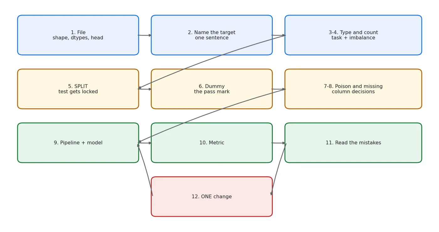
12 steps. The last arrow goes back to step 9: it is a loop, not a straight line.
Notice that the last arrow goes back. ML is a loop, not a checklist you run once. You go round 9→12 dozens of times.
What we learned today
show(pd.DataFrame([
    {"Step": "1-4", "In one sentence": "Understand the data without touching a model"},
    {"Step": "5", "In one sentence": "Lock the test set away (this is where leakage stops)"},
    {"Step": "6", "In one sentence": "Get the pass mark; without it you can't judge anything"},
    {"Step": "7-8", "In one sentence": "Drop the poisonous columns, handle the missing values"},
    {"Step": "9", "In one sentence": "ONE simple model in a Pipeline"},
    {"Step": "10", "In one sentence": "Choose the metric that fits the task"},
    {"Step": "11", "In one sentence": "Read the rows it got wrong; the next step comes from there"},
    {"Step": "12", "In one sentence": "ONE change and back to step 9"},
]))
| Step | In one sentence |
|---|---|
| 1-4 | Understand the data without touching a model |
| 5 | Lock the test set away (this is where leakage stops) |
| 6 | Get the pass mark; without it you can't judge anything |
| 7-8 | Drop the poisonous columns, handle the missing values |
| 9 | ONE simple model in a Pipeline |
| 10 | Choose the metric that fits the task |
| 11 | Read the rows it got wrong; the next step comes from there |
| 12 | ONE change and back to step 9 |
Our results:
show(pd.DataFrame([
    {"Model": "Dummy (baseline)", "Accuracy": f"{baseline:.4f}", "Note": "Learned nothing"},
    {"Model": "Logistic + Pipeline", "Accuracy": f"{acc:.4f}", "Note": "+0.27 over the baseline"},
    {"Model": "+ 2 new features", "Accuracy": f"{acc_new:.4f}", "Note": "Almost no change, an honest result"},
    {"Model": "+ agent_komissiyasi", "Accuracy": f"{acc_leak:.4f}", "Note": "LEAKAGE, a false result"},
]))
| Model | Accuracy | Note |
|---|---|---|
| Dummy (baseline) | 0.5056 | Learned nothing |
| Logistic + Pipeline | 0.7778 | +0.27 over the baseline |
| + 2 new features | 0.7833 | Almost no change, an honest result |
| + agent_komissiyasi | 1.0000 | LEAKAGE, a false result |
The card for your desk
card = """
+--------------------------------------------------------------+
|  A NEW DATASET: 12 STEPS                                     |
+--------------------------------------------------------------+
|   1  shape, dtypes, head()                                   |
|   2  "I predict ___ from ___"                                |
|   3  target type -> regression / classification              |
|   4  value_counts(normalize=True)  <- YOUR BASELINE          |
|   5  train_test_split(..., stratify=y)   NOW!                |
|   6  DummyClassifier -> write the pass mark down             |
|   7  nunique() -> IDs;  "will I have it?" -> leakage         |
|   8  isna().sum();  object columns -> OneHot                 |
|   9  ColumnTransformer -> Pipeline -> fit                    |
|  10  confusion_matrix, precision, recall, F1                 |
|  11  READ the wrong rows (nlargest by confidence)            |
|  12  ONE change -> back to step 9                            |
+--------------------------------------------------------------+
|  A perfect result (>0.99) = a leakage signal, not a party    |
|  Without the baseline, accuracy means nothing                |
|  The test set is in the safe: it gets opened once            |
+--------------------------------------------------------------+
"""
print(card)
+--------------------------------------------------------------+
|  A NEW DATASET: 12 STEPS                                     |
+--------------------------------------------------------------+
|   1  shape, dtypes, head()                                   |
|   2  "I predict ___ from ___"                                |
|   3  target type -> regression / classification              |
|   4  value_counts(normalize=True)  <- YOUR BASELINE          |
|   5  train_test_split(..., stratify=y)   NOW!                |
|   6  DummyClassifier -> write the pass mark down             |
|   7  nunique() -> IDs;  "will I have it?" -> leakage         |
|   8  isna().sum();  object columns -> OneHot                 |
|   9  ColumnTransformer -> Pipeline -> fit                    |
|  10  confusion_matrix, precision, recall, F1                 |
|  11  READ the wrong rows (nlargest by confidence)            |
|  12  ONE change -> back to step 9                            |
+--------------------------------------------------------------+
|  A perfect result (>0.99) = a leakage signal, not a party    |
|  Without the baseline, accuracy means nothing                |
|  The test set is in the safe: it gets opened once            |
+--------------------------------------------------------------+
Next chapter
You just walked the whole path once. If you didn't understand everything, that's normal. The rest of the book goes deeper into each of the twelve steps:
| Step | Which chapter |
|---|---|
| 1–4 (looking at the data) | Chapter 3 SQL, Chapter 4 visualisation |
| 5 (split, leakage) | Chapter 6 |
| 6 (baseline) | Chapter 7 |
| 7–8 (cleaning) | Chapter 5 |
| 9 (models) | Chapters 15–22 |
| 10 (metrics) | Chapters 8, 9, 10 |
| 11 (error analysis) | Chapter 11 |
| 12 (decision) | Chapters 23–26 |
And in Chapter 42 I open a real Kaggle dataset for the first time and walk through it with all my mistakes left in.
Questions about this chapter?
The course, homework review and the other five books are in Uzbek. Questions in English are welcome on Telegram.