Support Vector Machine (SVM)
The scene: the widest street
We need to draw a line separating two classes. But infinitely many lines do the job: which one do you choose?
Logistic regression (Chapter 16) gives one answer, a tree (Chapter 18) gives another. SVM sets a precise criterion:
I find the WIDEST street between the two classes, and I draw the line down the middle of it.
The width of the street is the margin. The points touching its edges are the support vectors. That's where the name comes from.
What the margin is and why it matters
import pandas as pd
import numpy as np
import matplotlib.pyplot as plt
from sklearn.svm import SVC, LinearSVC
from sklearn.datasets import make_blobs

X_d, y_d = make_blobs(n_samples=60, centers=2, cluster_std=1.1, random_state=7)

svm = SVC(kernel="linear", C=1000).fit(X_d, y_d)   # large C = a hard margin
w, b0 = svm.coef_[0], svm.intercept_[0]

figure, ax = plt.subplots(figsize=(9, 5.5))
ax.scatter(X_d[:, 0], X_d[:, 1], c=y_d, cmap="coolwarm", s=45, edgecolors="k", linewidths=.5)
xx = np.linspace(X_d[:, 0].min() - 1, X_d[:, 0].max() + 1, 100)
yy = -(w[0] * xx + b0) / w[1]
edge = 1 / np.linalg.norm(w)
ax.plot(xx, yy, "k-", lw=2, label="decision line")
ax.plot(xx, yy + edge * np.sqrt(1 + (w[0]/w[1])**2), "k--", lw=1, label="margin edge")
ax.plot(xx, yy - edge * np.sqrt(1 + (w[0]/w[1])**2), "k--", lw=1)
ax.scatter(svm.support_vectors_[:, 0], svm.support_vectors_[:, 1],
           s=260, facecolors="none", edgecolors="green", linewidths=2.2,
           label=f"support vectors ({len(svm.support_vectors_)})")
ax.legend(fontsize=9); ax.set_title("SVM: the widest street", fontweight="bold")
ax.grid(alpha=.3)
fig("svm_margin.png", caption="The black line is the decision boundary. The dashed lines are the margin edges. The green circles are the support vectors.")

print(f"Total points    : {len(X_d)}")
print(f"Support vectors : {len(svm.support_vectors_)}")
print(f"Margin width    : {2/np.linalg.norm(w):.4f}")
Total points    : 60
Support vectors : 3
Margin width    : 3.9591
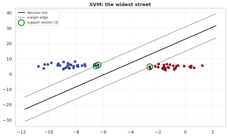
The black line is the decision boundary. The dashed lines are the margin edges. The green circles are the support vectors.
Notice: only a few of the 60 points define the model. Delete the other points and the line doesn't change.
# proof: we remove everything except the support vectors
sv_idx = svm.support_
svm2 = SVC(kernel="linear", C=1000).fit(X_d[sv_idx], y_d[sv_idx])
print(f"On all the data    : w = {svm.coef_[0].round(4)}, b = {svm.intercept_[0]:.4f}")
print(f"On the SVs only    : w = {svm2.coef_[0].round(4)}, b = {svm2.intercept_[0]:.4f}")
print(f"The same           : {bool(np.allclose(svm.coef_, svm2.coef_, atol=1e-3))}")
On all the data    : w = [ 0.4893 -0.1257], b = 2.8536
On the SVs only    : w = [ 0.4892 -0.126 ], b = 2.8549
The same           : True
Why this is theoretically elegant
The widest margin is the most reliable boundary. Even if a new point is shifted a little, the wide street keeps it on the right side.
That's why SVM generalises well on small data: it doesn't depend on every point in the data, only on the points at the boundary.
Column names
The rental data below has Uzbek column names. xonalar rooms, maydon_m2 area in m², qavat floor, qavatlar_soni floors in the building, metro_km distance to the metro, mebel furnished (0/1). The target ijaraga_berildi_30k means rented within 30 days.
The C parameter: hard and soft margins
In real data the classes don't separate cleanly. So SVM allows some points into the street, with a penalty.
C is the strength of that penalty.
from sklearn.model_selection import train_test_split, cross_val_score
from sklearn.pipeline import Pipeline
from sklearn.preprocessing import StandardScaler

df = pd.read_csv(DATA / "uy_ijara.csv")
num = ["xonalar", "maydon_m2", "qavat", "qavatlar_soni", "metro_km", "mebel"]
X, y = df[num], df["ijaraga_berildi_30k"]
X_tr, X_te, y_tr, y_te = train_test_split(X, y, test_size=0.3, random_state=42, stratify=y)

print(f"{'C':>8} {'margin':>10} {'SV count':>9} {'CV F1':>9} {'note'}")
print("-" * 54)
for C in [0.01, 0.1, 1, 10, 100]:
    q = Pipeline([("sc", StandardScaler()), ("m", SVC(kernel="linear", C=C))]).fit(X_tr, y_tr)
    b = cross_val_score(Pipeline([("sc", StandardScaler()), ("m", SVC(kernel="linear", C=C))]),
                        X, y, cv=5, scoring="f1")
    m = q.named_steps["m"]
    note = "soft margin" if C <= 0.1 else ("hard margin" if C >= 100 else "")
    print(f"{C:>8} {'wide' if C <= 0.1 else 'narrow':>10} {m.n_support_.sum():>9} {b.mean():>9.4f} {note}")
       C     margin  SV count     CV F1 note
------------------------------------------------------
    0.01       wide       625    0.7242 soft margin
     0.1       wide       590    0.7247 soft margin
       1     narrow       583    0.7233
      10     narrow       583    0.7239
     100     narrow       584    0.7239 hard margin
show(pd.DataFrame([
    {"C": "small (0.01-0.1)", "Margin": "WIDE", "Attitude to errors": "Tolerates them",
     "Result": "A simpler model, many support vectors", "Risk": "Underfitting"},
    {"C": "large (100+)", "Margin": "NARROW", "Attitude to errors": "Punishes them hard",
     "Result": "A complex boundary, few support vectors", "Risk": "Overfitting"},
]))
| C | Margin | Attitude to errors | Result | Risk |
|---|---|---|---|---|
| small (0.01-0.1) | WIDE | Tolerates them | A simpler model, many support vectors | Underfitting |
| large (100+) | NARROW | Punishes them hard | A complex boundary, few support vectors | Overfitting |
C has the SAME logic as the C in Chapter 17
We said in Chapter 17: in LogisticRegression(C=...), C = 1/alpha.
SVM is exactly the same: large C = WEAK regularisation.
So Ridge(alpha=100) and SVC(C=0.01) both mean "a strong penalty". To avoid mixing them up, remember: alpha raises the penalty, C lowers it.
The kernel trick: SVM's superpower
So far we used kernel="linear". But SVM's real strength lies elsewhere.
Remember the ring data from Chapter 16? The linear model got 0.5350.
r = np.random.default_rng(42)
n = 600
angle = r.uniform(0, 2 * np.pi, n)
radius = np.where(r.random(n) < 0.5, r.normal(1, .25, n), r.normal(3, .3, n))
Xh = np.c_[radius * np.cos(angle), radius * np.sin(angle)]
yh = (radius > 2).astype(int)

from sklearn.linear_model import LogisticRegression
from sklearn.tree import DecisionTreeClassifier

print(f"{'model':<34} {'CV accuracy':>13} {'±':>8}")
print("-" * 58)
for name, m in [
    ("LogisticRegression (Chapter 16)", LogisticRegression()),
    ("DecisionTree (Chapter 18)", DecisionTreeClassifier(max_depth=6, random_state=42)),
    ("SVM kernel='linear'", SVC(kernel="linear")),
    ("SVM kernel='rbf'", SVC(kernel="rbf")),
]:
    b = cross_val_score(Pipeline([("sc", StandardScaler()), ("m", m)]), Xh, yh, cv=5)
    print(f"{name:<34} {b.mean():>13.4f} {b.std():>8.4f}")
model                                CV accuracy        ±
----------------------------------------------------------
LogisticRegression (Chapter 16)           0.5350   0.0220
DecisionTree (Chapter 18)                 0.9883   0.0085
SVM kernel='linear'                       0.6400   0.0266
SVM kernel='rbf'                          1.0000   0.0000
kernel="rbf" separated the ring almost perfectly, by changing one parameter.
How? The kernel moves the data into a higher dimension, where the classes separate linearly, then brings the result back. And it does this without actually moving anything: it just computes the dot products differently. That's why it's called a "trick".
show(pd.DataFrame([
    {"Kernel": "linear", "When": "Many columns, text data (TF-IDF)",
     "Parameters": "C", "Speed": "Fast"},
    {"Kernel": "rbf", "When": "THE DEFAULT CHOICE: when you need a complex boundary",
     "Parameters": "C, gamma", "Speed": "Slower"},
    {"Kernel": "poly", "When": "When a polynomial relationship is known",
     "Parameters": "C, degree, gamma", "Speed": "Slow"},
    {"Kernel": "sigmoid", "When": "Rarely used",
     "Parameters": "C, gamma", "Speed": "Slow"},
]))
| Kernel | When | Parameters | Speed |
|---|---|---|---|
| linear | Many columns, text data (TF-IDF) | C | Fast |
| rbf | THE DEFAULT CHOICE: when you need a complex boundary | C, gamma | Slower |
| poly | When a polynomial relationship is known | C, degree, gamma | Slow |
| sigmoid | Rarely used | C, gamma | Slow |
gamma: the radius of the rbf kernel
print(f"{'gamma':>10} {'CV accuracy':>13} {'note'}")
print("-" * 48)
for g in [0.001, 0.01, 0.1, 1, 10, 100]:
    b = cross_val_score(Pipeline([("sc", StandardScaler()), ("m", SVC(kernel="rbf", gamma=g))]),
                        Xh, yh, cv=5)
    note = "very smooth (underfit)" if g <= 0.001 else ("every point its own island (overfit)" if g >= 100 else "")
    print(f"{g:>10} {b.mean():>13.4f} {note}")
print()
print("'scale' (the default) is chosen automatically from the data's variance:")
b = cross_val_score(Pipeline([("sc", StandardScaler()), ("m", SVC(kernel='rbf', gamma='scale'))]), Xh, yh, cv=5)
print(f"  gamma='scale'  CV accuracy = {b.mean():.4f}")
     gamma   CV accuracy note
------------------------------------------------
     0.001        0.5033 very smooth (underfit)
      0.01        0.5383
       0.1        1.0000
         1        1.0000
        10        0.9967
       100        0.9767 every point its own island (overfit)

'scale' (the default) is chosen automatically from the data's variance:
  gamma='scale'  CV accuracy = 1.0000
gamma sets each support vector's "radius of influence":
- small gamma: a large radius, a smooth boundary
- large gamma: a small radius, every point guards its own surroundings (overfitting)
C and gamma must be tuned TOGETHER
They're linked: a large C + a large gamma = guaranteed overfitting.
So for SVM, GridSearchCV searches the two together (Chapter 24):
{"m__C": [0.1, 1, 10, 100], "m__gamma": [0.001, 0.01, 0.1, 1]}
That's 16 combinations: that's what tuning SVM costs.
Scaling is vital for SVM
print("SVM, with and without scaling:")
for name, m in [("no scaling", SVC()),
                ("scaling", Pipeline([("sc", StandardScaler()), ("m", SVC())]))]:
    b = cross_val_score(m, X, y, cv=5, scoring="f1")
    print(f"  {name:14s} CV F1 = {b.mean():.4f} ±{b.std():.4f}")
SVM, with and without scaling:
  no scaling     CV F1 = 0.7263 ±0.0056
  scaling        CV F1 = 0.7308 ±0.0135
The reason is the same as for KNN (Chapter 21): SVM relies on distances, so a large-scale column drowns out everything else.
Speed: SVM's main limitation
import time
from sklearn.datasets import make_classification

print(f"{'rows':>10} {'SVC (rbf)':>12} {'LinearSVC':>12} {'LogisticReg':>13}")
print("-" * 52)
for n_q in [500, 2000, 8000]:
    Xb, yb = make_classification(n_samples=n_q, n_features=20, n_informative=10, random_state=42)
    row = [f"{n_q:>10}"]
    for m in [SVC(kernel="rbf"), LinearSVC(dual="auto", max_iter=5000), LogisticRegression(max_iter=2000)]:
        t0 = time.perf_counter()
        Pipeline([("sc", StandardScaler()), ("m", m)]).fit(Xb, yb)
        row.append(f"{(time.perf_counter()-t0)*1000:>11.0f}ms")
    print(" ".join(row))
      rows    SVC (rbf)    LinearSVC   LogisticReg
----------------------------------------------------
       500           3ms           1ms           4ms
      2000          26ms           2ms           2ms
      8000         255ms           7ms           6ms
Look at the table: as the rows grow, SVC's time shoots up.
The reason: kernel SVM's complexity is between
show(pd.DataFrame([
    {"Rows": "< 10 000", "Choice": "SVC(kernel='rbf')", "Note": "You can use the kernel's power"},
    {"Rows": "10 000 - 100 000", "Choice": "LinearSVC or SGDClassifier", "Note": "A kernel is too expensive"},
    {"Rows": "> 100 000", "Choice": "LogisticRegression / LightGBM", "Note": "SVM doesn't fit at all"},
]))
| Rows | Choice | Note |
|---|---|---|
| < 10 000 | SVC(kernel='rbf') | You can use the kernel's power |
| 10 000 - 100 000 | LinearSVC or SGDClassifier | A kernel is too expensive |
| > 100 000 | LogisticRegression / LightGBM | SVM doesn't fit at all |
SVM was king in the 2010s, not today
Before deep learning, SVM was considered the strongest model. Today, on tabular data, boosting (Chapter 20) beats it almost every time, and runs faster.
Where SVM still fits:
- Small data (hundreds of rows): few parameters, good generalisation
- More columns than rows (m > n): genetics, text
- Text classification with TF-IDF: LinearSVC is still a strong baseline
On a new project, start with boosting or logistic regression as your first choice.
Probability: SVM doesn't give probabilities
svc = Pipeline([("sc", StandardScaler()), ("m", SVC())]).fit(X_tr, y_tr)
try:
    svc.predict_proba(X_te[:3])
except AttributeError as e:
    print("SVC().predict_proba() ->", type(e).__name__)
    print(f"  {str(e)[:70]}")
print()
svc_p = Pipeline([("sc", StandardScaler()), ("m", SVC(probability=True, random_state=42))]).fit(X_tr, y_tr)
print("With probability=True:")
print(f"  {svc_p.predict_proba(X_te[:3])[:, 1].round(4)}")
print()
print("decision_function: SVM's NATURAL output (the distance from the boundary):")
print(f"  {svc.decision_function(X_te[:3]).round(4)}")
SVC().predict_proba() -> AttributeError
  This 'Pipeline' has no attribute 'predict_proba'

With probability=True:
  [0.2973 0.771  0.7154]

decision_function: SVM's NATURAL output (the distance from the boundary):
  [-0.9156  1.2765  0.9675]
probability=True is expensive
SVM doesn't naturally give probabilities: it only gives the distance from the boundary.
Set probability=True and sklearn runs 5-fold cross-validation internally to train Platt calibration. Training time goes up about 5 times.
For moving the threshold (Chapter 9), decision_function() is enough: it also gives an ordered score.
The variants
show(pd.DataFrame([
    {"Class": "SVC", "Task": "Classification", "Kernel": "Yes", "When": "n < 10 000"},
    {"Class": "LinearSVC", "Task": "Classification", "Kernel": "No (linear only)", "When": "Large n, text"},
    {"Class": "SVR", "Task": "Regression", "Kernel": "Yes", "When": "Small regression"},
    {"Class": "LinearSVR", "Task": "Regression", "Kernel": "No", "When": "Large regression"},
    {"Class": "OneClassSVM", "Task": "Anomaly detection", "Kernel": "Yes", "When": "When you only have 'normal' data"},
]))
| Class | Task | Kernel | When |
|---|---|---|---|
| SVC | Classification | Yes | n < 10 000 |
| LinearSVC | Classification | No (linear only) | Large n, text |
| SVR | Regression | Yes | Small regression |
| LinearSVR | Regression | No | Large regression |
| OneClassSVM | Anomaly detection | Yes | When you only have 'normal' data |
The end of Part 4: every algorithm in one table
from sklearn.ensemble import RandomForestClassifier
from sklearn.neighbors import KNeighborsClassifier
from sklearn.naive_bayes import GaussianNB
from xgboost import XGBClassifier

print(f"{'model':<28} {'CV F1':>9} {'±':>8} {'scaling':>9}")
print("-" * 60)
results = []
for name, m, needs_sc in [
    ("LogisticRegression (16)", LogisticRegression(max_iter=2000), True),
    ("DecisionTree (18)", DecisionTreeClassifier(max_depth=6, min_samples_leaf=20, random_state=42), False),
    ("RandomForest (19)", RandomForestClassifier(n_estimators=200, random_state=42), False),
    ("XGBoost (20)", XGBClassifier(n_estimators=200, verbosity=0, random_state=42), False),
    ("KNN (21)", KNeighborsClassifier(n_neighbors=15), True),
    ("GaussianNB (21)", GaussianNB(), False),
    ("SVM rbf (22)", SVC(), True),
]:
    pipe = Pipeline([("sc", StandardScaler()), ("m", m)]) if needs_sc else m
    b = cross_val_score(pipe, X, y, cv=5, scoring="f1")
    results.append((name, b.mean(), b.std()))
    print(f"{name:<28} {b.mean():>9.4f} {b.std():>8.4f} {'yes' if needs_sc else 'no':>9}")

print()
best = max(results, key=lambda x: x[1])
spread = max(n[2] for n in results)
close = [n[0] for n in results if best[1] - n[1] < spread]
print(f"Highest          : {best[0]} ({best[1]:.4f})")
print(f"Within the spread: {len(close)} models -> {', '.join(close)}")
model                            CV F1        ±   scaling
------------------------------------------------------------
LogisticRegression (16)         0.7210   0.0111       yes
DecisionTree (18)               0.6715   0.0246        no
RandomForest (19)               0.6824   0.0185        no
XGBoost (20)                    0.6715   0.0292        no
KNN (21)                        0.7064   0.0191       yes
GaussianNB (21)                 0.7291   0.0080        no
SVM rbf (22)                    0.7308   0.0135       yes

Highest          : SVM rbf (22) (0.7308)
Within the spread: 4 models -> LogisticRegression (16), KNN (21), GaussianNB (21), SVM rbf (22)
Pay attention to the last line. By the Chapter 10 rule, the gap between models within the spread is not reliable.
Our data is small (1200 rows) and easy. So complex models don't beat simple ones, which is a very common situation in practice.
What we learned today
show(pd.DataFrame([
    {"Concept": "Margin", "In one sentence": "The widest street between the two classes"},
    {"Concept": "Support vectors", "In one sentence": "Only the points at the boundary define the model"},
    {"Concept": "C", "In one sentence": "Large C = narrow margin = weak regularisation"},
    {"Concept": "The kernel trick", "In one sentence": "A non-linear boundary without moving to a higher dimension"},
    {"Concept": "gamma", "In one sentence": "A support vector's radius of influence; tuned together with C"},
    {"Concept": "Scaling", "In one sentence": "REQUIRED: it relies on distances"},
    {"Concept": "Speed", "In one sentence": "O(n^2)-O(n^3): no good beyond 10 000 rows"},
    {"Concept": "Probability", "In one sentence": "Not natural; probability=True is 5x the cost"},
]))
| Concept | In one sentence |
|---|---|
| Margin | The widest street between the two classes |
| Support vectors | Only the points at the boundary define the model |
| C | Large C = narrow margin = weak regularisation |
| The kernel trick | A non-linear boundary without moving to a higher dimension |
| gamma | A support vector's radius of influence; tuned together with C |
| Scaling | REQUIRED: it relies on distances |
| Speed | O(n^2)-O(n^3): no good beyond 10 000 rows |
| Probability | Not natural; probability=True is 5x the cost |
That completes Part 4. You've seen eight algorithms and you know when each one fits.
But the most important conclusion is a different one: on your data, many of them give the same result. So choosing the algorithm is a small part of the work. The main work is in the data (Part 1), the evaluation (Part 2) and the error analysis (Chapter 11).
Questions about this chapter?
The course, homework review and the other five books are in Uzbek. Questions in English are welcome on Telegram.